MV-2050: Linear Analysis for Stability and Vibration Analysis
In this tutorial, you will learn how to perform a linear analysis using MotionView and MotionSolve. You will also learn how to interpret its results and use the same for improving the stability of your systems.
In this tutorial you will use a simplified quarter model of a bus represented by a two degrees of freedom system consisting of masses suspended by two springs. Next, you can optionally apply the concepts to perform a similar study using a real-life model of a full car provided here that makes some practical sense.
Open and Review the Simplified Quarter Bus Model
-
Click on Open Model,
 ,
from the Standard toolbar.
,
from the Standard toolbar.
-
Review the bodies present in the model.
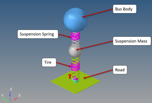
Figure 1. Simplified Bus Model Setup -
Review the properties of spring dampers respresenting the Tire and
SuspensionSpring connections.
Note: The figure below shows the properties of SuspensionSpring.
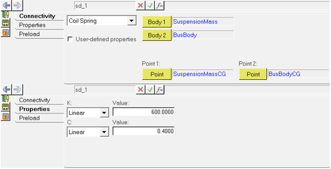
Figure 2. Spring_Damper Properties of SuspensionSpring
Determine Natural Frequencies
A linear analysis can be run on system to determine its natural frequencies and mode shapes.
-
Review the linear analysis system available in the model.
Note: There is a motion provided on the joint that connects Road with the Ground Body as shown in the figure below. Check its properties; 0 mm constant value locks this joint in its initial position.
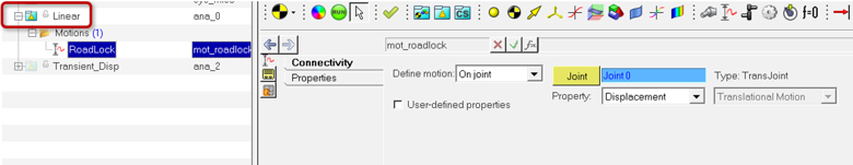
Figure 3. Motion to Lock Road Movement -
Go to the Run panel
 and rename the XML file to
SimplifiedTwoSpring_Model_Linear.xml.
Make sure that Simulation type and Analysis are both set to Static+Linear on the Run panel.
and rename the XML file to
SimplifiedTwoSpring_Model_Linear.xml.
Make sure that Simulation type and Analysis are both set to Static+Linear on the Run panel. -
Click the Simulation Settings button and choose the
Linear tab from the dialog to turn on the
Disable damping option as shown in the figure
below.
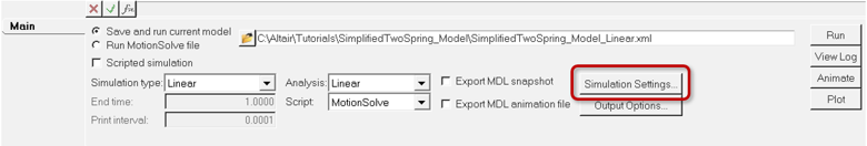
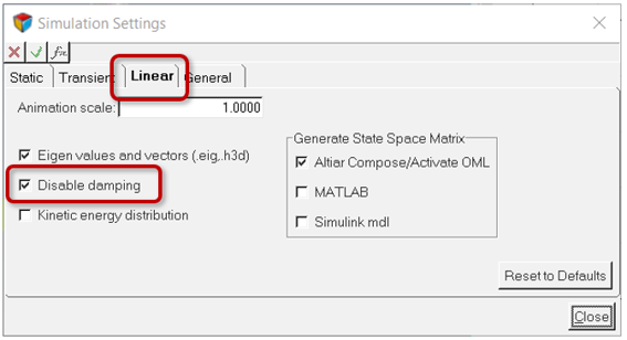
Figure 4. Settings for Linear AnalysisNote: The natural frequency of a system does not depend on damping. Disabling damping will simply remove its contribution in the complex eigenvalue analysis. You may want to keep the default settings and observe how the results differ. -
Once the run is complete, review the solver window and observe the natural
frequencies determined by the solver as shown in the figure below.
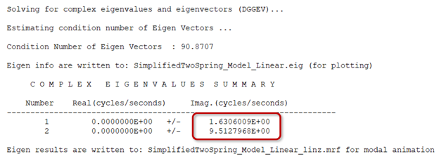
Figure 5. Natural Frequencies Identified by the MotionSolve Run -
Once the H3D file is loaded in HyperView, click the
Start/Pause Animation button
 and then choose the modes from the drop-down menu
available in the Results Browser to view the mode shapes as
shown in the figure below.
and then choose the modes from the drop-down menu
available in the Results Browser to view the mode shapes as
shown in the figure below.
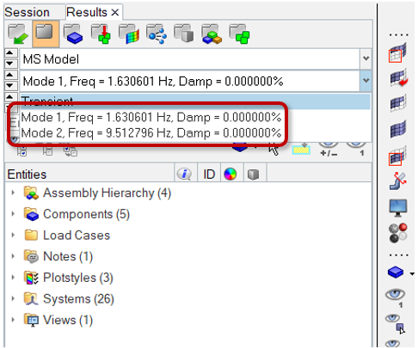
Figure 6. Plot Mode Shapes in HyperViewNote: It is evident that Mode 1 involves major contribution of the BusBody vibration, while Mode 2 has major contribution of the SupsensionMass vibration. -
Pause the animation
 and return to the MotionView window when you are done.
Response to External Excitation
In this step a small enforced displacement in the form of a sinusoidal excitation on the road is applied at different frequencies to determine the response of the system. Here an expression of the form sin(2*π*f*t) is used, where ‘f’ is the natural frequency of the sine curve and ‘t’ is time.
- Excitation at a frequency away from the natural frequency (in other words, 4Hz)
- Excitation at a natural frequency (in other words, First mode at ~ 1.63Hz)
- Excitation over a range of frequencies (from 0Hz to 10Hz)
-
Right-click on the Transient_Disp analysis available in
the model and choose Activate > Selected object(s) and
review the same.
Note: This should automatically deactivate the Linear analysis, since only one analysis can be active at a time in the model. Refer to the figure below.
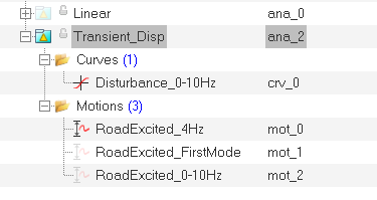
Figure 7. Transient Analysis -
Next, right-click on the RoadExcited_4Hz and choose
Activate > Selected object(s).
This applies a sine-based motion on Road with an amplitude of 1mm at a frequency of 4Hz (away from natural frequency of the system) as shown in figure below.
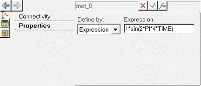
Figure 8. Harmonic Excitation on Road -
Go to the Run panel and rename the XML file to
SimplifiedTwoSpring_Model_4Hz.xml.
-
Make sure that Simulation type is set to
Static+Transient and Analysis is set to
Transient_Disp on the Run panel.
Note: As shown in the figure below; observe that a very small Print interval of 0.001 is chosen to accurately measure the outputs. Review the value of Maximum step size by clicking the Simulation Settings button and choosing the Transient tab from the dialog. It has been changed from a default value of 0.01 to make it the same as that of the print interval. If this is not done, the solver will enforce the same during the run to be able to write the output at the desired frequency.
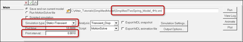
Figure 9. Run Panel Settings -
Plot the displacement over time for BusBody, SuspensionMass and Road using the
following settings as shown in the table below.
Body Y Request SuspensionMass REQ/70000000 SuspensionDisp- (on SuspensionMass) - DZ BusBody REQ/70000002 BusBodyDisp- (on BusBody) - DZ Road REQ/70000004 RoadDisp- (on Road) - DZ Note: Use following settings for all plots as shown in the figure below:- X Type: Time
- Y Type: Marker Displacement
- Y Component: Dz
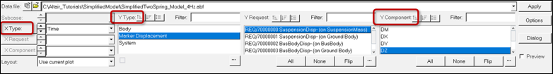
Figure 10. HyperGraph Settings for PlotsObtain the plots as shown in the figure below. Observe that the amplitude tends to reduce over time suggesting that the system is going to attain stability. This is due to the damping present in the springs of the system. Thus, this external excitation of small amplitude at frequency of 4Hz may not be harmful.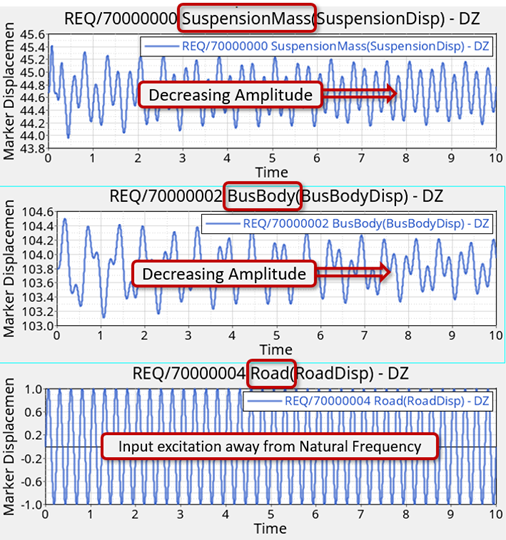
Figure 11. System Response Away from Natural Frequency -
Repeat steps #2 to #8 with the next motion in the analysis,
RoadExcited_FirstMode.
Note: This motion uses the natural frequency of system as obtained from Linear analysis performed earlier.
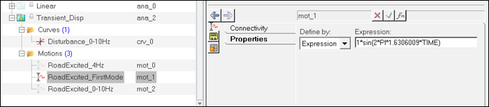
Figure 12. External Excitation at First ModeObtain the plots as shown in the figure below. Observe that the amplitude tends to increase over time suggesting that the system is going out of control even in the presence of damping in the springs. This demonstrates the phenomena of resonance which can be detrimental and result in system failure.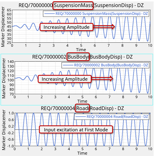
Figure 13. System Response at First Mode -
Again, repeat steps #2 to #8 with the next motion in the analysis,
RoadExcited_0-10Hz.
Note: This is a curve-based motion of constant amplitude and variable frequency within the range of 0Hz to 10Hz. This range includes both the natural frequencies of system as identified by Linear analysis.
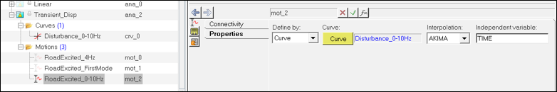
Figure 14.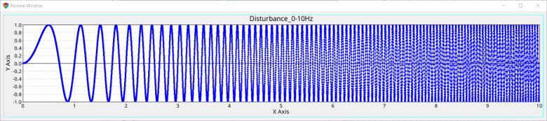
Figure 15.Obtain the plots as shown in the figure below.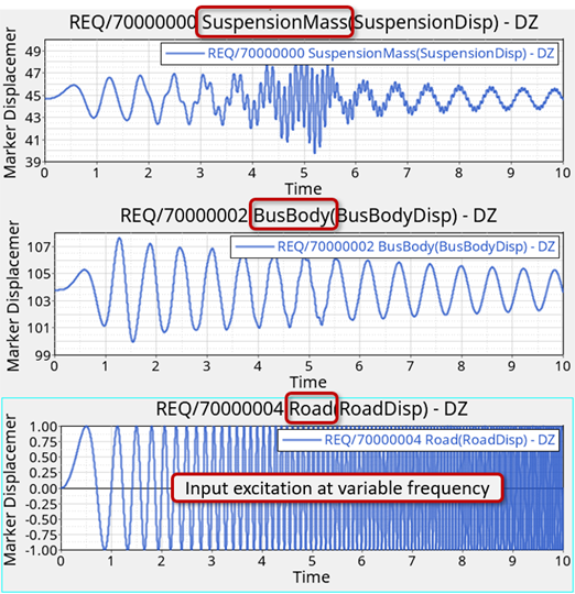
Figure 16. System Response at Variable FrequencyThese plots may not make much sense until the data is converted into frequency domain. To do so, follow the steps outlined in Step 4 Convert Output to Frequency Domain (below).
Convert Output to Frequency Domain
In this step the SuspensionMass displacement output plotted with respect to time will be used and plotted with respect to frequency using the Hanning type of Fourier Transforms.
-
In HyperGraph, click on the Load Preference File button
and select the Vehicle Safety Tools preference
file.
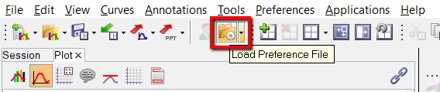
Figure 17. -
Add an additional window using the Page Window Layout
button and select it to make it active.
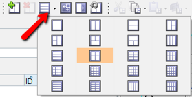
Figure 18. -
From the Transforms menu, select Fourier Transforms >
Hanning.
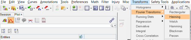
Figure 19. -
Perform the following actions to generate the plot.
-
Keep the Shift key on the keyboard pressed.
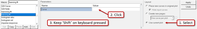
Figure 20. -
Observe the plotted curve.
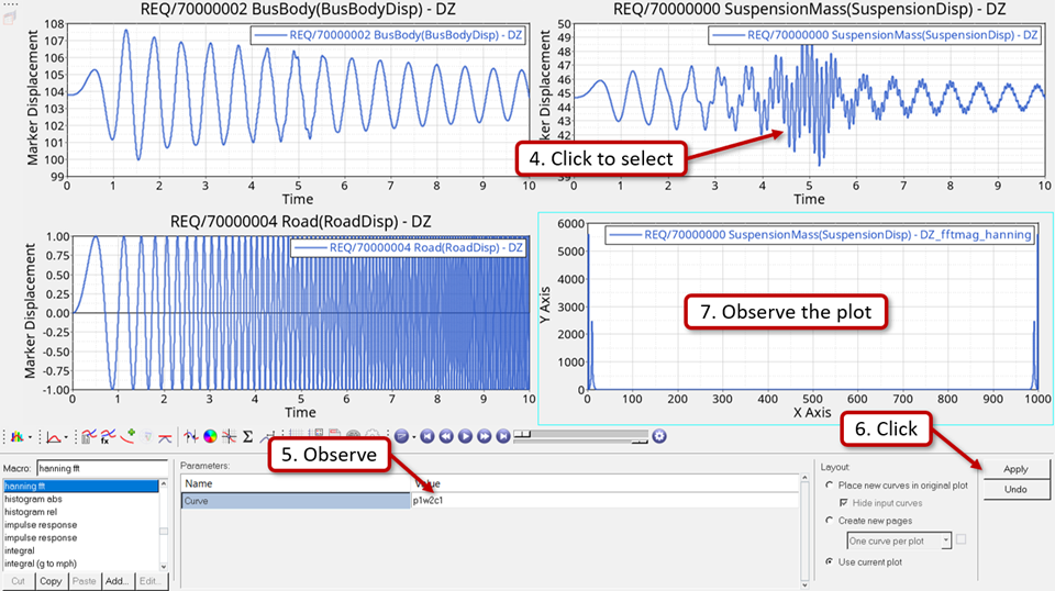
Figure 21. -
Select the Logarithmic scale.
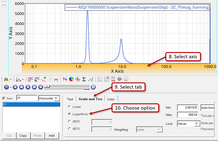
Figure 22.
-
Keep the Shift key on the keyboard pressed.
Study the Full Vehicle Model (optional)
A full car model has been provided with this tutorial as described earlier.
-
Unzip the FullCar_Linear.zip file in your
<working directory>.
The model should look like the one shown in the figure below.
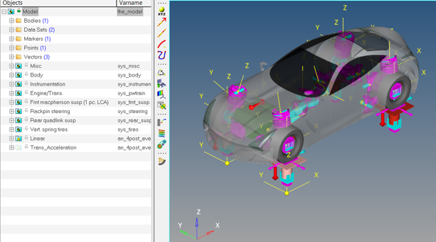
Figure 23. Full Car Model -
The model contains engine vibration measured using an accelerometer from the
ignition to idle throttle as shown in the figure below.
The engine at idle throttle runs at ~1000rpm.
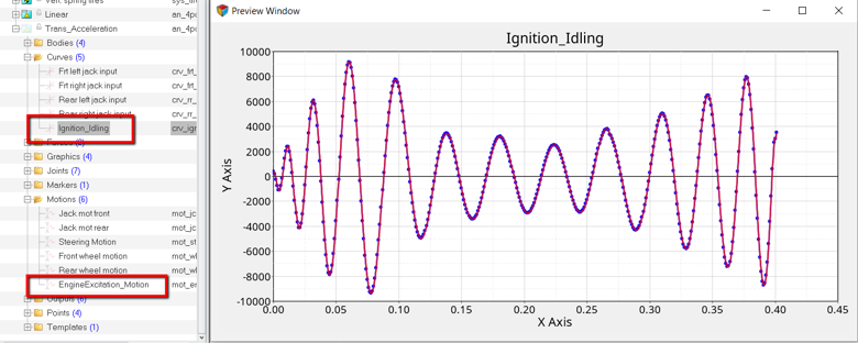
Figure 24. Engine Acceleration During Ignition to Idle Throttle -
The steering wheel of the car has been mounted on a flexible bushing block as
shown in the figure below.
It is important to make sure that its natural frequency is away from the engine’s idling frequency to avoid unwanted vibrations.
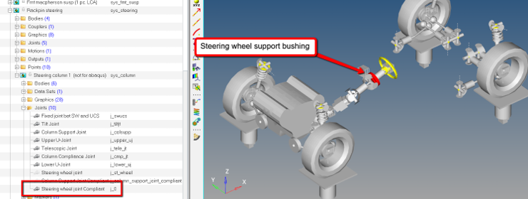
Figure 25. Steering Wheel Support -
The figure below shows the steering wheel’s natural frequency as identified by
linear analysis. This is very near to engine’s idling frequency (~15Hz).
Try changing the steering wheel support’s bushing stiffness to shift it out of the idling frequency range (0-15hz).
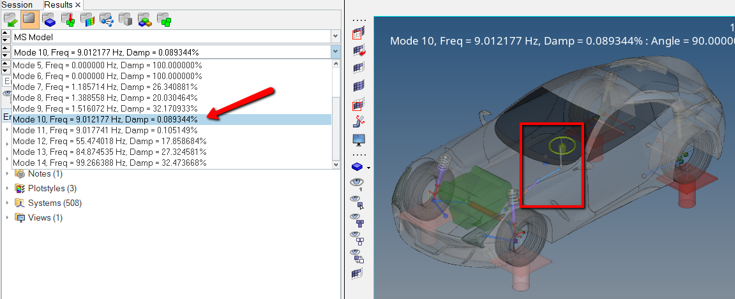
Figure 26. Steering Wheel Support