OS-T: 9000 OptiStruct and VABS Integration

The structural FEA solver OptiStruct and VABS are integrated on the Altair Simulation platform to analyze slender structures via the latter’s ability to compute the complete set of beam section properties for an arbitrary cross-sectional shape and material without any ad hoc kinematic assumptions.

HyperMesh remains the primary preprocessing tool to generate input for VABS.

VABS (Variational Asymptotic Beam Sectional Analysis) is a cross-sectional analysis tool for computing 1D beam properties and recovering 3D stresses/strains of slender composite structures (and also isotropic materials).

With this enhancement in OptiStruct and Altair Simulation framework, users can perform Analysis of composite beams in a single seamless run of OptiStruct, where VABS is invoked internally. The VABS libraries can be downloaded from Altair Connect.
Note: On Altair Connect, there are two VABS versions available for download, and for OptiStruct-VABS Integration, the VABS version to be chosen will be named “VABS-# Packaged with OptiStruct”, where # is the version number of the VABS software.
The downloaded VABS libraries should then be placed in the OptiStruct installation directories at the following locations:
  • For Windows:

    <install_directory>\hwsolvers\optistruct\lib\win64\VABS

  • For Linux:

    <install_directory>/hwsolvers/optistruct/lib/linux64/VABS

The HyperMesh interface has special utility to generate a finite element mesh of the cross section including all the details of geometry and material as inputs to calculate the sectional properties including structural properties and inertial properties. VABS compatible input file is saved at a prescribed working directory. The unified work flow further enables to generate OptiStruct input deck for the residual model in the same HyperMesh session.

With the ASSIGN command, OptiStruct identifies the VABS inputs, solves and generate equivalent stiffness matrix by invoking the VABS executable. OptiStruct further reads VABS output and executes the full solver run.


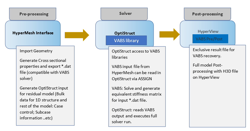
Figure 1. High Level Workflow
In this tutorial, a composite pipe with uniform thickness is considered. The ply sequencing and orientation are:


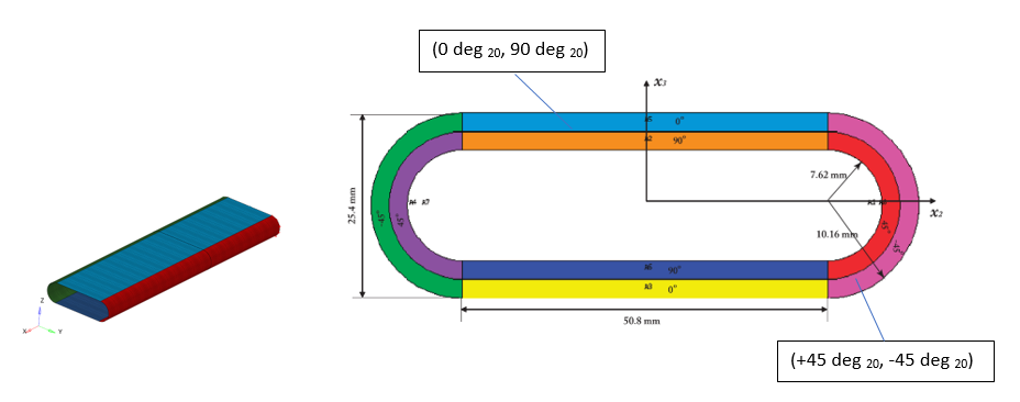
Figure 2. Composite Pipe
Orthotropic material with ply orientations (in degrees) as:
  • E11 = 141.693
  • E22 = E33 = 9.79056 (GPa)
  • G12 = G23 = G31 = 5.99844e9 (GPa)
  • v 12 MathType@MTEF@5@5@+= feaagKart1ev2aaatCvAUfeBSjuyZL2yd9gzLbvyNv2CaerbuLwBLn hiov2DGi1BTfMBaeXatLxBI9gBaerbd9wDYLwzYbItLDharqqtubsr 4rNCHbGeaGqiVu0Je9sqqrpepC0xbbL8F4rqqrFfpeea0xe9Lq=Jc9 vqaqpepm0xbba9pwe9Q8fs0=yqaqpepae9pg0FirpepeKkFr0xfr=x fr=xb9adbaqaaeGaciGaaiaabeqaamaabaabaaGcbaGaamODamaaBa aaleaacaaIXaGaaGOmaaqabaaaaa@3894@ = v 23 MathType@MTEF@5@5@+= feaagKart1ev2aaatCvAUfeBSjuyZL2yd9gzLbvyNv2CaerbuLwBLn hiov2DGi1BTfMBaeXatLxBI9gBaerbd9wDYLwzYbItLDharqqtubsr 4rNCHbGeaGqiVu0Je9sqqrpepC0xbbL8F4rqqrFfpeea0xe9Lq=Jc9 vqaqpepm0xbba9pwe9Q8fs0=yqaqpepae9pg0FirpepeKkFr0xfr=x fr=xb9adbaqaaeGaciGaaiaabeqaamaabaabaaGcbaGaamODamaaBa aaleaacaaIXaGaaGOmaaqabaaaaa@3894@ = v 31 MathType@MTEF@5@5@+= feaagKart1ev2aaatCvAUfeBSjuyZL2yd9gzLbvyNv2CaerbuLwBLn hiov2DGi1BTfMBaeXatLxBI9gBaerbd9wDYLwzYbItLDharqqtubsr 4rNCHbGeaGqiVu0Je9sqqrpepC0xbbL8F4rqqrFfpeea0xe9Lq=Jc9 vqaqpepm0xbba9pwe9Q8fs0=yqaqpepae9pg0FirpepeKkFr0xfr=x fr=xb9adbaqaaeGaciGaaiaabeqaamaabaabaaGcbaGaamODamaaBa aaleaacaaIXaGaaGOmaaqabaaaaa@3894@ = 0.42
1D elements (CBEAM) are idealized along the center of the pipe, such that the beam axis is aligned to the X-axis of the pipe. A total number of 25 CBEAM elements are chosen for better convergence.


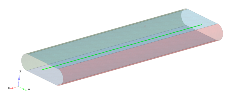
Figure 3. 1D (CBEAM) Elements Aligned with the x-axis Center of the Composite Pipe

Launch HyperMesh and Set the Profiles

The model shown in Figure 3 is used in this exercise. The 2D (SHELL) mesh and 1D (CBEAM) elements are already idealized.

  1. Launch HyperMesh Desktop.
    The User Profile dialog opens.
  2. For Application, select Engineering Solutions.
  3. Toggle Aerospace-OptiStruct and click OK.

Open the Model

  1. Click File > Open > Model.
  2. Select the osVABS_example.hm file you saved to your working directory from the optistruct.zip file. Refer to Access the Model Files.
  3. Click Open.
  4. In the Model Browser, right-click Review on the Properties folder, to visiualize the property assignment and ply layout.

    Review the two properties: wall_top_bottom and wall_sides.

  5. Click on either property.
  6. In the Entity Editor, expand Number of Plies.
  7. Click on the table editor to review the ply sequencing and orientation.

Set Up the Model

Update Section Properties for VABS and Create *.dat File

The special utility is opened to create the section properties for the given cross-section and export VABS input file to the working directory.

  1. Click Aerospace > Beams > Beams from lines.
    The Beam Tool dialog opens.
  2. For Action, select Update under Value from the drop-down menu.
  3. For Entities, click on the 0 Elements and then click on the yellow Elements button.
    This allows you to select elements from the panel.
  4. From the panel, click on the yellow elems button.
  5. Select by id and select any one 1D (CBEAM) element from the graphics window (choose element ID: 5761 for the exercise problem).
  6. Click Proceed.
  7. For Property/Sections, click the check box next to Update Section/Property.
  8. For Section, click in the Value field, and select Elements from the drop-down menu.
    This should enable to choose elements from the panel (similar to step above).
  9. Click on Elements > By Collector, from the panel, and select the four components which contain shell elements (pipe_top; pipe_bottom; pipe_right; pipe_left).
  10. Click Proceed.
  11. Under Export VABS, specify the location where the VABS input file (*.dat) is to be exported.


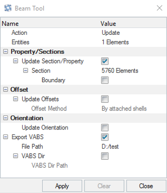
    Figure 4. Define Settings in the Beam Tool Dialog
  12. Click Apply.
    This should generate the shell mesh at the plane of cross-section for visualization purpose only.


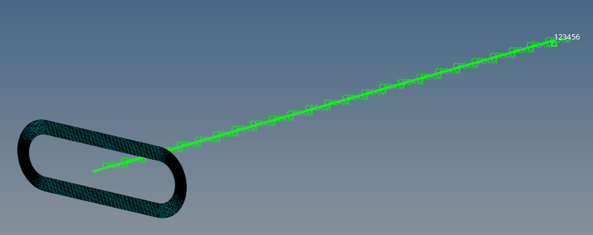
    Figure 5. Visualization of the Shell Mesh at the Cross-section
  13. Click Close to close the Beam Tool dialog.
    A user warning window displays to clear the section graphics (section mesh).
  14. Click Yes.

Update Components

  1. In the Model Browser, expand the Components folder.
  2. Right-click on the beam component and click Assign.
    An Assign to Components dialog opens.
  3. Select the newly created property Beam_ID_Vabs_5761_Prop.
  4. Click Apply and OK.


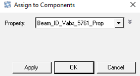
    Figure 6. Assign Property to Beam Component
    Note:
    • As the thickness is uniform in this exercise, a section property was created for only one CBEAM elment (element ID: 5761) and then you assigned the newly created beam property to rest of the 24 CBEAM elements (Step 2).
    • Multiple cross-sections should be created, if there is a change in the cross-section of the pipe.
    • The Beam Tool generates separate cross section for every CBEAM element selected and hence a separate VABS input file (*.dat) is generated, if multiple CBEAM elements are selected in Step 3.
  5. In the Model Browser, expand Components folder.
  6. Select the four components which contain shell elements (pipe_top; pipe_bottom; pipe_right; and pipe_left).
  7. Right-click and select Delete.

Define Materials

On the MAT8 entry, E2 and NU12, and HyperMesh, are defined by default, currently exports E3, NU13 and NU23 as zero in the *.dat file. Therefore, you will manually set the following data in the *.dat file.

  1. In a text editor, open the *.dat file you saved in Step 4.
  2. Scroll to the very end of the *.dat file to locate:
    1.41963000e+11  9.79056000e+09  0.00000000e+00
    5.99844000e+09  5.99844000e+09  5.99844000e+09
    4.20000000e-01  0.00000000e+00  0.00000000e+00
  3. Manually edit to read as:
    1.41963000e+11  9.79056000e+09  9.79056000e+09
    5.99844000e+09  5.99844000e+09  5.99844000e+09
    4.20000000e-01  4.20000000e-01  4.20000000e-01
    Note: Default settings for E3, NU13, and NU23, as mentioned above will be automated in a future version of HyperMesh.

Review Cross-section Property and ASSIGN Card

  1. In the Model Browser, expand the Properties folder.
  2. Right-click on Beam_ID_Vabs_5761_Prop.
  3. Click Card Edit to review the Group and Type of the PBEAML.
    1. Verify Group is set to VABS.
    2. Type is set to Vabs5761 (suffix of the element ID of the CBEAM chosen for generating cross section).


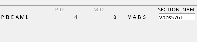
      Figure 7. Review PBEAML VABS Property
  4. In the Model Browser, expand Cards folder.
  5. Right-click on ASSIGN.
  6. In the Entity Editor, verify:
    1. Type is set to VABS.
    2. Section_Name is set to Vabs5761.
    3. Section_Path is set to the directory where the VABS input *.dat has to be exported.


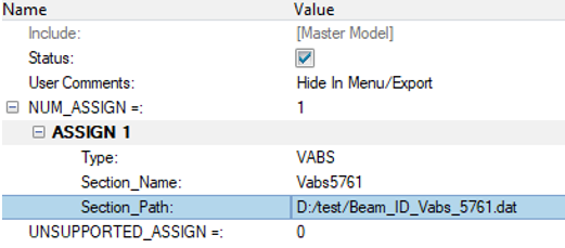
      Figure 8. Review the ASSIGN Entry

Create Load Collector

The boundary conditions for the Modal Analysis are defined here.

  1. In the Model Browser, right-click and select Create > Load Collector.
  2. For Name, enter SPC.
  3. For Card Image, select NONE.
  4. From the toolbar, select BCs > Create > Constraints.
  5. Select the node ID: 1, and check all the dofs from 1 to 6.
  6. Click create.
    An SPC at node 1 on the CBEAM element is created.
  7. Click Esc key to exit the constraint creation panel.
  8. In the Model Browser, right-click and select Create > Load Collector.
  9. For Name, enter Eigen.
  10. For Card Image, select EIGRL.
  11. For ND, enter 10.

Create Loadstep

You will define the modal loadcase in this step.

  1. In the Model Browser, right-click and select Create > Load Step.
  2. For Name, enter ModeShapes.
  3. For Analysis type, select Normal modes.
  4. For SPC, select SPC from the list of the load collectors.
  5. For Method (STRUCT), select Eigen.
    The modal analysis loadcase is created.

Submit the Job

  1. From the Analysis page, click OptiStruct.
  2. Click save as following the input file: field.
    A Save As dialog opens.
  3. For File name, enter osVabs_example.fem.
  4. The input file: field is set to the location of osVabs_example.fem.
  5. Click Save.
  6. Click OptiStruct to submit the analysis.

Review the Results

OptiStruct automatically invokes the VABS executables and runs the *.dat file to generate equivalent stiffness matrix. OptiStruct reads VABS output and executes full solver run.

  1. When the analysis process completes, click HyperView to launch the results.
  2. In the Results tab, select Subcase 1 (ModeShapes) from the subcase field.
  3. Go to the Contour panel in HyperView.
  4. For Result type, select Eigen Mode(v).
  5. Click Apply to visualize the contour plot.
    Different modes could be contoured by changing the mode number under the Subcase.


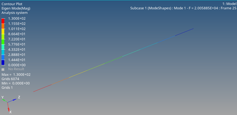
    Figure 9. Mode Shape Results in HyperView

    Unlike isotropic beams, composite beams exhibit strong coupling between various types of deformation – in this case extension-twist and bending-shear couplings, which is evident from the mode shapes.