This tutorial demonstrates a phone drop test simulation using Explicit Analysis in
OptiStruct when the phone is dropped on the floor with a
velocity of 5425 mm/s.
The exercises in this tutorial are:
Set up the explicit drop test model in HyperMesh
Submit the job in OptiStruct
View the results in HyperView
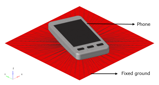
Figure 1 illustrates the structural model used for this
tutorial. The phone and its parts are considered in this model. The phone is dropped
on the floor at a velocity of 5425 mm/s. Figure 1. Model and Loading Description
Launch HyperMesh and Set the OptiStruct User Profile
Launch HyperMesh.
The User Profile dialog opens.
Select OptiStruct and click
OK.
This loads the user profile. It includes the appropriate template, macro
menu, and import reader, paring down the functionality of HyperMesh to what is relevant for generating models for
OptiStruct.
Open the Model
Click File > Open > Model.
Select the Drop_test_phone.hm file you saved to
your working directory from the optistruct.zip file. Refer
to Access the Model Files.
Click Open.
The Drop_test_phone.hm database is loaded
into the current HyperMesh session, replacing any
existing data.
Apply Loads and Boundary Conditions
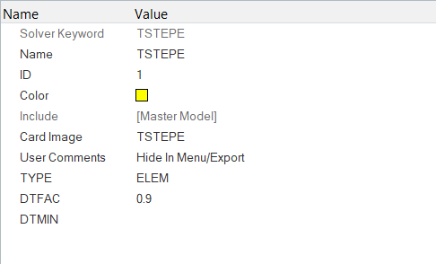
Create TSTEPE Load Collector
The time-step control parameters for explicit analysis is defined.
In the Model Browser, right-click and select Create > Load Collector.
For Name, enter TSTEPE.
For Card image, select TSTEPE.
For TYPE, select ELEM.
for DTFAC, enter 0.9.
Figure 2. TSTEPE Definition
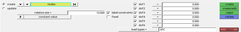
Create SPC Load Collector
In this step, Single Point Constraints (SPCs) is used to fix the floor.
In the Model Browser, right-click and select Create > Load Collector.
For Name, enter SPC.
From the main menu, click BCs > Create > Constraints to open the Constraints panel.
Select the independent node of the RBE2 element and select all DOFs (1 through
6), and enter a value of 0 (all the DOFs are
fixed).
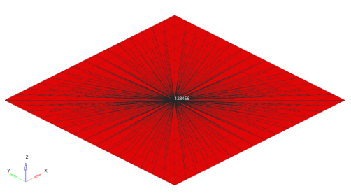
Figure 3. Definition of SPC on the selected node Figure 4. SPC applied to for floor
Click Create > return.
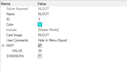
Create NLOUT Load Collector
In the Model Browser, right-click and select Create > Load Collector.
For Name, enter NLOUT.
For Card Image, select NLOUT from the drop-down
menu.
Activate NINT, then for VALUE, enter 30.
Figure 5. NLOUT Definition
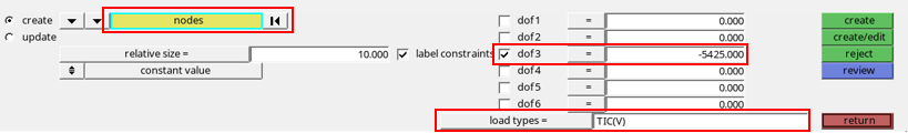
Create INI_VEL Load Collector
In this step, an initial velocity of 5425 mm/s will be applied to the phone in the
negative Z direction.
In the Model Browser, right-click and select Create > Load Collector.
For Name, enter INI_VEL.
Click BCs > Create > Constraints to open the Constraints panel.
Activate the create radio button.
Toggle to nodes and click on
nodes and select by
sets.
Select phone_nodes set and click
select.
This Set is already created in the model.
For load types =, select TIC(V).
Activate only dof3 and enter
-5425.0.
Figure 6. Definition of Initial Velocity
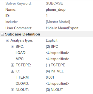
Create Explicit Load Step
In this step, an explicit load step will be created, where the previously defined
load collectors will be referenced.
In the Model Browser, right-click and select Create > Load Step.
For Name, enter phone_drop.
Under Subcase Definition, Analysis type, select
Explicit.
For SPC, select SPC and click
OK.
For TSTEPE, select TSTEPE and click
OK.
For IC, select INI_VEL and click
OK.
For TTERM, enter 0.001.
For NLOUT, select NLOUT and click
OK.
Figure 7. Create Explicit Load Step
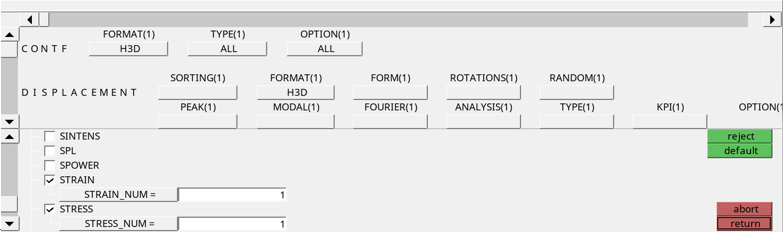
Add Control Cards
In this step, control cards for the simulation will be defined.
Select Analysis > control cards.
Click next to advance until
GLOBAL_OUTPUT_REQUEST is available, then click
GLOBAL_OUTPUT_REQUEST.
Activate the CONTF checkbox.
For FORMAT, select H3D.
For OPTION, select ALL.
Activate the DISPLACEMENT checkbox.
For FORMAT, select H3D.
For OPTION, select ALL.
Activate the STRESS checkbox.
For FORMAT, select H3D.
For OPTION, select ALL.
Activate the STRAIN checkbox.
For FORMAT, select H3D.
For OPTION, select ALL.
Figure 8. Definition of Control Cards
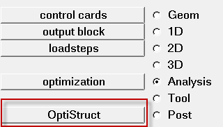
Submit the Job
From the Analysis page, click the OptiStruct
panel.
Figure 9. Accessing the OptiStruct Panel
Click save as.
In the Save As dialog, specify the location to write the
OptiStruct model file and enter
Drop_test.fem for the filename.
For OptiStruct input decks,
.fem is the recommended extension.
Click save.
The input file field displays the filename and location specified in the
save As dialog.
Set export options to all.
Set run options to analysis.
Set memory options to memory default.
Click OptiStruct to launch
the OptiStruct job.
If the job is successful, new results files
should be in the directory where the Drop_test.fem was written. The
Drop_test.out file is a good place to look for error messages
that could help debug the input deck if any errors are present.
Review the Results
View a contour plot of stresses and displacement.
From the OptiStruct panel, click HyperView.
HyperView is launched and the results are
loaded. A message window appears to inform of the successful model and result
files loading into HyperView.
Go to the Results tab.
On the Results toolbar, click to open the
Contour panel.
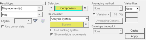
Set Result type to Displacement and click on
Apply to contour the elements.
Figure 10. Set Displacement as Result Type
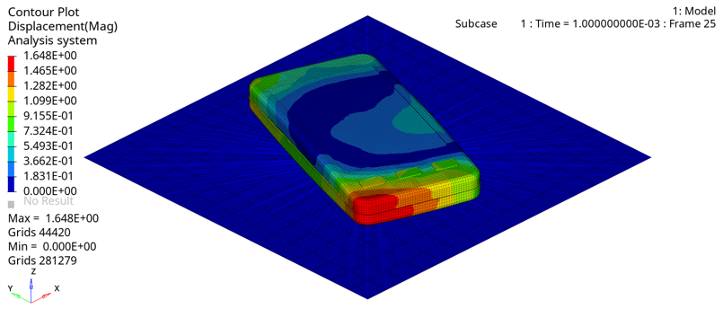
The contour of displacement plot is observed at the final increment. Figure 11. Displacement Contour
 to open the
Contour panel.
to open the
Contour panel.