The shock tube problem is one of the standard problems in gas dynamics. It is a very
interesting test since the exact solution is known and can be compared with the simulation
results. The Finite Element method using the Eulerian and Lagrangian formulations was used
in the numerical models.
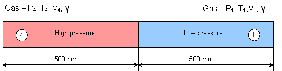
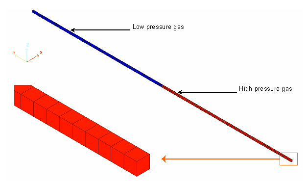
A shock tube consists of a long tube filled with the same gas in two different physical states.
The tube is divided into two parts, separated by a diaphragm. The initial state is
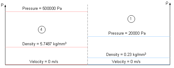
defined by the values for density, pressure and velocity, as shown in
Figure 2 and
Figure 3 . All the viscous effects are negligible along
the tube sides; it is also assumed that there is no motion in the beginning.
Figure 2. Shock Tube Sketch
Figure 3. Initial States with Discontinuities
The initial state at time t = 0 consists of two constant states 1 and 4 with
p
4
>
p
1
ρ
4
>
ρ
1
v
4
=
v
1
= 0
MathType@MTEF@5@5@+=
feaagKart1ev2aqatCvAUfeBSjuyZL2yd9gzLbvyNv2CaerbuLwBLn
hiov2DGi1BTfMBaeXatLxBI9gBaerbd9wDYLwzYbItLDharqqtubsr
4rNCHbGeaGqiVu0Je9sqqrpepC0xbbL8F4rqqrFfpeea0xe9Lq=Jc9
vqaqpepm0xbbG8FasPYRqj0=yi0dXdbba9pGe9xq=JbbG8A8frFve9
Fve9Ff0dmeaabaqaciGacaGaaeqabaWaaeaaeaaakeaacaWG2bWaaS
baaSqaaiaaisdaaeqaaOGaeyypa0JaamODamaaBaaaleaacaaIXaaa
beaakiabg2da9iaaicdaaaa@3D00@
Table 1. Initial Conditions in the Shock Tube
High Pressure Side
(4)
Low Pressure Side
(1)
Pressure
p
500000
[
Pa ]
20000
[
Pa ]
Velocity
v
MathType@MTEF@5@5@+=
feaagKart1ev2aqatCvAUfeBSjuyZL2yd9gzLbvyNv2CaerbuLwBLn
hiov2DGi1BTfMBaeXatLxBI9gBaerbd9wDYLwzYbItLDharqqtubsr
4rNCHbGeaGqiVu0Je9sqqrpepC0xbbL8F4rqqrFfpeea0xe9Lq=Jc9
vqaqpepm0xbbG8FasPYRqj0=yi0dXdbba9pGe9xq=JbbG8A8frFve9
Fve9Ff0dmeaabaqaciGacaGaaeqabaWaaeaaeaaakeaacaWG2baaaa@375A@
0
[
m
s
]
MathType@MTEF@5@5@+=
feaagKart1ev2aaatCvAUfeBSjuyZL2yd9gzLbvyNv2CaerbuLwBLn
hiov2DGi1BTfMBaeXatLxBI9gBaerbd9wDYLwzYbItLDharqqtubsr
4rNCHbGeaGqiVu0Je9sqqrpepC0xbbL8F4rqqrFfpeea0xe9Lq=Jc9
vqaqpepm0xbba9pwe9Q8fs0=yqaqpepae9pg0FirpepeKkFr0xfr=x
fr=xb9adbaqaaeGaciGaaiaabeqaamaabaabaaGcbaWaamWaaeaada
Wcaaqaaiaab2gaaeaacaqGZbaaaaGaay5waiaaw2faaaaa@39DE@
Density
ρ
5.7487
[
k
g
m
m
3
]
MathType@MTEF@5@5@+=
feaagKart1ev2aqatCvAUfeBSjuyZL2yd9gzLbvyNv2CaerbuLwBLn
hiov2DGi1BTfMBaeXatLxBI9gBaerbd9wDYLwzYbItLDharqqtubsr
4rNCHbGeaGqiVu0Je9sqqrpepC0xbbL8F4rqqrFfpeea0xe9Lq=Jc9
vqaqpepm0xbbG8FasPYRqj0=yi0dXdbba9pGe9xq=JbbG8A8frFve9
Fve9Ff0dmeaabaqaciGacaGaaeqabaWaaeaaeaaakeaadaWadaqaam
aalaaabaGaai4AaiaacEgaaeaacaGGTbGaaiyBamaaCaaaleqabaGa
ai4maaaaaaaakiaawUfacaGLDbaaaaa@3D0B@
0.22995
[
k
g
m
m
3
]
MathType@MTEF@5@5@+=
feaagKart1ev2aqatCvAUfeBSjuyZL2yd9gzLbvyNv2CaerbuLwBLn
hiov2DGi1BTfMBaeXatLxBI9gBaerbd9wDYLwzYbItLDharqqtubsr
4rNCHbGeaGqiVu0Je9sqqrpepC0xbbL8F4rqqrFfpeea0xe9Lq=Jc9
vqaqpepm0xbbG8FasPYRqj0=yi0dXdbba9pGe9xq=JbbG8A8frFve9
Fve9Ff0dmeaabaqaciGacaGaaeqabaWaaeaaeaaakeaadaWadaqaam
aalaaabaGaai4AaiaacEgaaeaacaGGTbGaaiyBamaaCaaaleqabaGa
ai4maaaaaaaakiaawUfacaGLDbaaaaa@3D0B@
Temperature
T
303
[
K
]
303
[
K
]
Just after the membrane is removed, a compression shock runs into the low pressure region, while a rarefaction (decompression) wave moves into the high pressure part of the tube. Furthermore, a contact discontinuity usually occurs.
Model Method
The hydrodynamic viscous fluid LAW6 is used to describe compressed gas.
The general equation describing pressure is:
(1)
p
=
C
0
+
C
1
μ
+
C
2
μ
2
+
C
3
μ
3
+
(
C
4
+
C
5
μ
)
E
MathType@MTEF@5@5@+=
feaagKart1ev2aqatCvAUfeBSjuyZL2yd9gzLbvyNv2CaerbuLwBLn
hiov2DGi1BTfMBaeXatLxBI9gBaerbd9wDYLwzYbItLDharqqtubsr
4rNCHbGeaGqiVu0Je9sqqrpepC0xbbL8F4rqqrFfpeea0xe9Lq=Jc9
vqaqpepm0xbbG8FasPYRqj0=yi0dXdbba9pGe9xq=JbbG8A8frFve9
Fve9Ff0dmeaabaqaciGacaGaaeqabaWaaeaaeaaakeaacaWGWbGaey
ypa0Jaam4qamaaBaaaleaacaaIWaaabeaakiabgUcaRiaadoeadaWg
aaWcbaGaaGymaaqabaGccqaH8oqBcqGHRaWkcaWGdbWaaSbaaSqaai
aaikdaaeqaaOGaeqiVd02aaWbaaSqabeaacaaIYaaaaOGaey4kaSIa
am4qamaaBaaaleaacaaIZaaabeaakiabeY7aTnaaCaaaleqabaGaaG
4maaaakiabgUcaRmaabmaabaGaam4qamaaBaaaleaacaaI0aaabeaa
kiabgUcaRiaadoeadaWgaaWcbaGaaGynaaqabaGccqaH8oqBaiaawI
cacaGLPaaacaWGfbaaaa@5235@
With
μ
=
ρ
ρ
0
−
1
MathType@MTEF@5@5@+=
feaagKart1ev2aaatCvAUfeBSjuyZL2yd9gzLbvyNv2CaerbuLwBLn
hiov2DGi1BTfMBaeXatLxBI9gBaerbd9wDYLwzYbItLDharqqtubsr
4rNCHbGeaGqiVu0Je9sqqrpepC0xbbL8F4rqqrFfpeea0xe9Lq=Jc9
vqaqpepm0xbba9pwe9Q8fs0=yqaqpepae9pg0FirpepeKkFr0xfr=x
fr=xb9adbaqaaeGaciGaaiaabeqaamaabaabaaGcbaGaeqiVd0Maey
ypa0ZaaSaaaeaacqaHbpGCaeaacqaHbpGCdaWgaaWcbaGaaGimaaqa
baaaaOGaeyOeI0IaaGymaaaa@3EDA@
Where,
p
Pressure
C
i
Hydrodynamic constants
E
n
Internal energy per initial volume
ρ
Density
Perfect gas is modeled by setting all coefficients:
(2)
C
0
=
C
1
=
C
2
=
C
3
=
0
MathType@MTEF@5@5@+=
feaagKart1ev2aaatCvAUfeBSjuyZL2yd9gzLbvyNv2CaerbuLwBLn
hiov2DGi1BTfMBaeXatLxBI9gBaerbd9wDYLwzYbItLDharqqtubsr
4rNCHbGeaGqiVu0Je9sqqrpepC0xbbL8F4rqqrFfpeea0xe9Lq=Jc9
vqaqpepm0xbba9pwe9Q8fs0=yqaqpepae9pg0FirpepeKkFr0xfr=x
fr=xb9adbaqaaeGaciGaaiaabeqaamaabaabaaGcbaGaam4qamaaBa
aaleaacaaIWaaabeaakiabg2da9iaadoeadaWgaaWcbaGaaGymaaqa
baGccqGH9aqpcaWGdbWaaSbaaSqaaiaaikdaaeqaaOGaeyypa0Jaam
4qamaaBaaaleaacaaIZaaabeaakiabg2da9iaaicdaaaa@41AE@
And
C
4
=
C
5
=
γ
−
1
Where,
γ
Then the initial internal energy, per initial volume is calculated from initial
pressure:
(3)
E
0
=
p
0
γ
−
1
MathType@MTEF@5@5@+=
feaagKart1ev2aqatCvAUfeBSjuyZL2yd9gzLbvyNv2CaerbuLwBLn
hiov2DGi1BTfMBaeXatLxBI9gBaerbd9wDYLwzYbItLDharqqtubsr
4rNCHbGeaGqiVu0Je9sqqrpepC0xbbL8F4rqqrFfpeea0xe9Lq=Jc9
vqaqpepm0xbbG8FasPYRqj0=yi0dXdbba9pGe9xq=JbbG8A8frFve9
Fve9Ff0dmeaabaqaciGacaGaaeqabaWaaeaaeaaakeaacaWGfbWaaS
baaSqaaiaaicdaaeqaaOGaeyypa0ZaaSaaaeaacaWGWbWaaSbaaSqa
aiaaicdaaeqaaaGcbaGaeq4SdCMaeyOeI0IaaGymaaaaaaa@3E63@
Under the assumption
γ
=
c
o
n
s
t
.
=
1.4
MathType@MTEF@5@5@+=
feaagKart1ev2aqatCvAUfeBSjuyZL2yd9gzLbvyNv2CaerbuLwBLn
hiov2DGi1BTfMBaeXatLxBI9gBaerbd9wDYLwzYbItLDharqqtubsr
4rNCHbGeaGqiVu0Je9sqqrpepC0xbbL8F4rqqrFfpeea0xe9Lq=Jc9
vqaqpepm0xbbG8FasPYRqj0=yi0dXdbba9pGe9xq=JbbG8A8frFve9
Fve9Ff0dmeaabaqaciGacaGaaeqabaWaaeaaeaaakeaacqaHZoWzcq
GH9aqpcaWGJbGaam4Baiaad6gacaWGZbGaamiDaiaac6cacqGH9aqp
caaIXaGaaiOlaiaaisdaaaa@41AF@
C
4
=
C
5
=
0.4
MathType@MTEF@5@5@+=
feaagKart1ev2aqatCvAUfeBSjuyZL2yd9gzLbvyNv2CaerbuLwBLn
hiov2DGi1BTfMBaeXatLxBI9gBaerbd9wDYLwzYbItLDharqqtubsr
4rNCHbGeaGqiVu0Je9sqqrpepC0xbbL8F4rqqrFfpeea0xe9Lq=Jc9
vqaqpepm0xbbG8FasPYRqj0=yi0dXdbba9pGe9xq=JbbG8A8frFve9
Fve9Ff0dmeaabaqaciGacaGaaeqabaWaaeaaeaaakeaacaWGdbWaaS
baaSqaaiaaisdaaeqaaOGaeyypa0Jaam4qamaaBaaaleaacaaI1aaa
beaakiabg2da9iaaicdacaGGUaGaaGinaaaa@3E0E@
Gas pressure is described by:
(4)
p
=
(
C
4
+
C
5
μ
)
E
MathType@MTEF@5@5@+=
feaagKart1ev2aqatCvAUfeBSjuyZL2yd9gzLbvyNv2CaerbuLwBLn
hiov2DGi1BTfMBaeXatLxBI9gBaerbd9wDYLwzYbItLDharqqtubsr
4rNCHbGeaGqiVu0Je9sqqrpepC0xbbL8F4rqqrFfpeea0xe9Lq=Jc9
vqaqpepm0xbbG8FasPYRqj0=yi0dXdbba9pGe9xq=JbbG8A8frFve9
Fve9Ff0dmeaabaqaciGacaGaaeqabaWaaeaaeaaakeaacaWGWbGaey
ypa0ZaaeWaaeaacaWGdbWaaSbaaSqaaiaaisdaaeqaaOGaey4kaSIa
am4qamaaBaaaleaacaaI1aaabeaakiabeY7aTbGaayjkaiaawMcaai
aadweaaaa@40BE@
(5)
p
=
(
0.4
+
0.4
ρ
−
ρ
0
ρ
0
)
E
MathType@MTEF@5@5@+=
feaagKart1ev2aqatCvAUfeBSjuyZL2yd9gzLbvyNv2CaerbuLwBLn
hiov2DGi1BTfMBaeXatLxBI9gBaerbd9wDYLwzYbItLDharqqtubsr
4rNCHbGeaGqiVu0Je9sqqrpepC0xbbL8F4rqqrFfpeea0xe9Lq=Jc9
vqaqpepm0xbbG8FasPYRqj0=yi0dXdbba9pGe9xq=JbbG8A8frFve9
Fve9Ff0dmeaabaqaciGacaGaaeqabaWaaeaaeaaakeaacaWGWbGaey
ypa0ZaaeWaaeaacaaIWaGaaiOlaiaaisdacqGHRaWkcaaIWaGaaiOl
aiaaisdadaWcaaqaaiabeg8aYjabgkHiTiabeg8aYnaaBaaaleaaca
aIWaaabeaaaOqaaiabeg8aYnaaBaaaleaacaaIWaaabeaaaaaakiaa
wIcacaGLPaaacaWGfbaaaa@4800@
(6)
E
0
=
p
0
0.4
MathType@MTEF@5@5@+=
feaagKart1ev2aqatCvAUfeBSjuyZL2yd9gzLbvyNv2CaerbuLwBLn
hiov2DGi1BTfMBaeXatLxBI9gBaerbd9wDYLwzYbItLDharqqtubsr
4rNCHbGeaGqiVu0Je9sqqrpepC0xbbL8F4rqqrFfpeea0xe9Lq=Jc9
vqaqpepm0xbbG8FasPYRqj0=yi0dXdbba9pGe9xq=JbbG8A8frFve9
Fve9Ff0dmeaabaqaciGacaGaaeqabaWaaeaaeaaakeaacaWGfbWaaS
baaSqaaiaaicdaaeqaaOGaeyypa0ZaaSaaaeaacaWGWbWaaSbaaSqa
aiaaicdaaeqaaaGcbaGaaGimaiaac6cacaaI0aaaaaaa@3D3E@
Parameters of material LAW6 are provided in Table 2 .
Table 2. Material Properties of Gas in LAW6
High Pressure Side
(4)
Low Pressure Side
(1)
Initial volumetric
energy density (E 0
1.25x10⁶
[
J
m
m
3
]
MathType@MTEF@5@5@+=
feaagKart1ev2aqatCvAUfeBSjuyZL2yd9gzLbvyNv2CaerbuLwBLn
hiov2DGi1BTfMBaeXatLxBI9gBaerbd9wDYLwzYbItLDharqqtubsr
4rNCHbGeaGqiVu0Je9sqqrpepC0xbbL8F4rqqrFfpeea0xe9Lq=Jc9
vqaqpepm0xbbG8FasPYRqj0=yi0dXdbba9pGe9xq=JbbG8A8frFve9
Fve9Ff0dmeaabaqaciGacaGaaeqabaWaaeaaeaaakeaadaWadaqaam
aalaaabaGaciOsaaqaaiaac2gacaGGTbWaaWbaaSqabeaacaGGZaaa
aaaaaOGaay5waiaaw2faaaaa@3C01@
5x10⁴
[
J
m
m
3
]
MathType@MTEF@5@5@+=
feaagKart1ev2aqatCvAUfeBSjuyZL2yd9gzLbvyNv2CaerbuLwBLn
hiov2DGi1BTfMBaeXatLxBI9gBaerbd9wDYLwzYbItLDharqqtubsr
4rNCHbGeaGqiVu0Je9sqqrpepC0xbbL8F4rqqrFfpeea0xe9Lq=Jc9
vqaqpepm0xbbG8FasPYRqj0=yi0dXdbba9pGe9xq=JbbG8A8frFve9
Fve9Ff0dmeaabaqaciGacaGaaeqabaWaaeaaeaaakeaadaWadaqaam
aalaaabaGaciOsaaqaaiaac2gacaGGTbWaaWbaaSqabeaacaGGZaaa
aaaaaOGaay5waiaaw2faaaaa@3C01@
C
4
C
5
0.4
0.4
Density
ρ
5.7487
[
k
g
m
m
3
]
MathType@MTEF@5@5@+=
feaagKart1ev2aqatCvAUfeBSjuyZL2yd9gzLbvyNv2CaerbuLwBLn
hiov2DGi1BTfMBaeXatLxBI9gBaerbd9wDYLwzYbItLDharqqtubsr
4rNCHbGeaGqiVu0Je9sqqrpepC0xbbL8F4rqqrFfpeea0xe9Lq=Jc9
vqaqpepm0xbbG8FasPYRqj0=yi0dXdbba9pGe9xq=JbbG8A8frFve9
Fve9Ff0dmeaabaqaciGacaGaaeqabaWaaeaaeaaakeaadaWadaqaam
aalaaabaGaai4AaiaacEgaaeaacaGGTbGaaiyBamaaCaaaleqabaGa
ai4maaaaaaaakiaawUfacaGLDbaaaaa@3D0B@
0.22995
[
k
g
m
m
3
]
MathType@MTEF@5@5@+=
feaagKart1ev2aqatCvAUfeBSjuyZL2yd9gzLbvyNv2CaerbuLwBLn
hiov2DGi1BTfMBaeXatLxBI9gBaerbd9wDYLwzYbItLDharqqtubsr
4rNCHbGeaGqiVu0Je9sqqrpepC0xbbL8F4rqqrFfpeea0xe9Lq=Jc9
vqaqpepm0xbbG8FasPYRqj0=yi0dXdbba9pGe9xq=JbbG8A8frFve9
Fve9Ff0dmeaabaqaciGacaGaaeqabaWaaeaaeaaakeaadaWadaqaam
aalaaabaGaai4AaiaacEgaaeaacaGGTbGaaiyBamaaCaaaleqabaGa
ai4maaaaaaaakiaawUfacaGLDbaaaaa@3D0B@
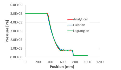
Analytical Approach
The shock tube problem has an analytical solution of time before the shock hits the
extremity of the tube.
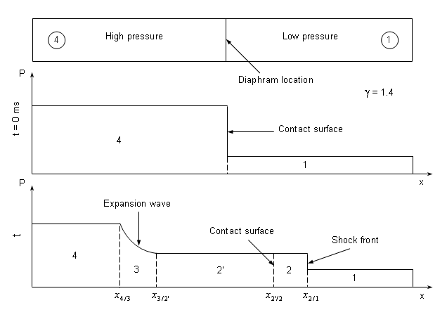
1
Figure 4. Schematic Shock Tube Problem with Pressure Distribution for
Pre- and Post-diaphragm Removal
Evolution of the flow pattern is illustrated in Figure 4 . When the diaphragm bursts, discontinuity
between the two initial states breaks into leftward and rightward moving waves,
separated by a contact surface.
Each wave pattern is composed of a contact discontinuity in the middle and a shock or
a rarefaction wave on the left and the right sides separating the uniform state
solution. The shock wave moves at a supersonic speed into the low pressure side. A
one-dimensional problem is considered.
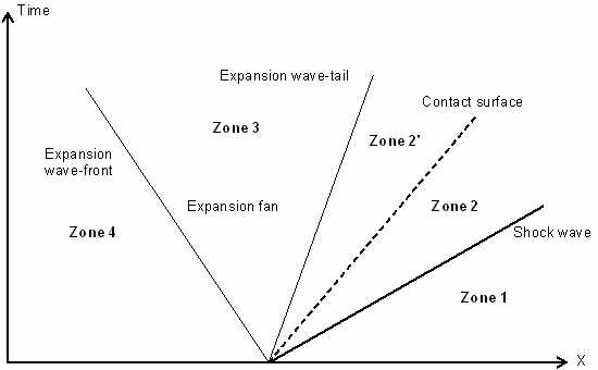
Figure 5. Shock Diagram, Expansion Waves and Contact Surface
There are four distinct zones marked 1, 2, 3 and 4 in
Figure 5 .
Zone 1 is the low pressure gas which is not disturbed by the shock wave.
Zone 2 (divided in 2 and 2' by the contact surface) contains the gas
immediately behind the shock traveling at a constant speed. The contact
surface across which the density and the temperature are discontinuous lies
within this zone.
The zone between the head and the tail of the expansion fan is noted as Zone
3. In this zone, the flow properties gradually change since the expansion
process is isentropic.
Zone 4 denotes the undisturbed high pressure gas.
Equations in Zone 2 are obtained using the normal shock relations. Pressure and the
velocity are constant in Zones 2 and 2'.
The ratio of the specific heat constant of gas
γ
The analytical solution to the Riemann problem is indicated at t=0.4 ms. A solution
is given according to the distinct zones and continuity must be checked. Evolution
in Zones 2 and 3 is dependent on the constant conditions of Zone 1 and 4. The
analytical equations use pressure, velocity, density, temperature, speed of sound
through gas and a specific gas constant. Equations in Zone 2 are obtained using
normal shock relations and the gas velocity in Zone 2 is constant throughout. The
shock wave and the surface contact speeds make it possible to define the position of
the zone limits.
Zone 4
Zone 1
Pressure
p
p
4
[
Pa ]
p
1
[
Pa ]
Velocity
v
MathType@MTEF@5@5@+=
feaagKart1ev2aqatCvAUfeBSjuyZL2yd9gzLbvyNv2CaerbuLwBLn
hiov2DGi1BTfMBaeXatLxBI9gBaerbd9wDYLwzYbItLDharqqtubsr
4rNCHbGeaGqiVu0Je9sqqrpepC0xbbL8F4rqqrFfpeea0xe9Lq=Jc9
vqaqpepm0xbbG8FasPYRqj0=yi0dXdbba9pGe9xq=JbbG8A8frFve9
Fve9Ff0dmeaabaqaciGacaGaaeqabaWaaeaaeaaakeaacaWG2baaaa@375A@
v
4
=
0
MathType@MTEF@5@5@+=
feaagKart1ev2aqatCvAUfeBSjuyZL2yd9gzLbvyNv2CaerbuLwBLn
hiov2DGi1BTfMBaeXatLxBI9gBaerbd9wDYLwzYbItLDharqqtubsr
4rNCHbGeaGqiVu0Je9sqqrpepC0xbbL8F4rqqrFfpeea0xe9Lq=Jc9
vqaqpepm0xbbG8FasPYRqj0=yi0dXdbba9pGe9xq=JbbG8A8frFve9
Fve9Ff0dmeaabaqaciGacaGaaeqabaWaaeaaeaaakeaacaWG2bWaaS
baaSqaaiaaisdaaeqaaOGaeyypa0JaaGimaaaa@3A0E@
[
m
s
]
MathType@MTEF@5@5@+=
feaagKart1ev2aaatCvAUfeBSjuyZL2yd9gzLbvyNv2CaerbuLwBLn
hiov2DGi1BTfMBaeXatLxBI9gBaerbd9wDYLwzYbItLDharqqtubsr
4rNCHbGeaGqiVu0Je9sqqrpepC0xbbL8F4rqqrFfpeea0xe9Lq=Jc9
vqaqpepm0xbba9pwe9Q8fs0=yqaqpepae9pg0FirpepeKkFr0xfr=x
fr=xb9adbaqaaeGaciGaaiaabeqaamaabaabaaGcbaWaamWaaeaada
Wcaaqaaiaab2gaaeaacaqGZbaaaaGaay5waiaaw2faaaaa@39DE@
v
1
=
0
MathType@MTEF@5@5@+=
feaagKart1ev2aqatCvAUfeBSjuyZL2yd9gzLbvyNv2CaerbuLwBLn
hiov2DGi1BTfMBaeXatLxBI9gBaerbd9wDYLwzYbItLDharqqtubsr
4rNCHbGeaGqiVu0Je9sqqrpepC0xbbL8F4rqqrFfpeea0xe9Lq=Jc9
vqaqpepm0xbbG8FasPYRqj0=yi0dXdbba9pGe9xq=JbbG8A8frFve9
Fve9Ff0dmeaabaqaciGacaGaaeqabaWaaeaaeaaakeaacaWG2bWaaS
baaSqaaiaaigdaaeqaaOGaeyypa0JaaGimaaaa@3A0B@
[
m
s
]
MathType@MTEF@5@5@+=
feaagKart1ev2aaatCvAUfeBSjuyZL2yd9gzLbvyNv2CaerbuLwBLn
hiov2DGi1BTfMBaeXatLxBI9gBaerbd9wDYLwzYbItLDharqqtubsr
4rNCHbGeaGqiVu0Je9sqqrpepC0xbbL8F4rqqrFfpeea0xe9Lq=Jc9
vqaqpepm0xbba9pwe9Q8fs0=yqaqpepae9pg0FirpepeKkFr0xfr=x
fr=xb9adbaqaaeGaciGaaiaabeqaamaabaabaaGcbaWaamWaaeaada
Wcaaqaaiaab2gaaeaacaqGZbaaaaGaay5waiaaw2faaaaa@39DE@
Density
ρ
ρ
4
[
k
g
m
m
3
]
MathType@MTEF@5@5@+=
feaagKart1ev2aqatCvAUfeBSjuyZL2yd9gzLbvyNv2CaerbuLwBLn
hiov2DGi1BTfMBaeXatLxBI9gBaerbd9wDYLwzYbItLDharqqtubsr
4rNCHbGeaGqiVu0Je9sqqrpepC0xbbL8F4rqqrFfpeea0xe9Lq=Jc9
vqaqpepm0xbbG8FasPYRqj0=yi0dXdbba9pGe9xq=JbbG8A8frFve9
Fve9Ff0dmeaabaqaciGacaGaaeqabaWaaeaaeaaakeaadaWadaqaam
aalaaabaGaai4AaiaacEgaaeaacaGGTbGaaiyBamaaCaaaleqabaGa
ai4maaaaaaaakiaawUfacaGLDbaaaaa@3D0B@
ρ
1
[
k
g
m
m
3
]
MathType@MTEF@5@5@+=
feaagKart1ev2aqatCvAUfeBSjuyZL2yd9gzLbvyNv2CaerbuLwBLn
hiov2DGi1BTfMBaeXatLxBI9gBaerbd9wDYLwzYbItLDharqqtubsr
4rNCHbGeaGqiVu0Je9sqqrpepC0xbbL8F4rqqrFfpeea0xe9Lq=Jc9
vqaqpepm0xbbG8FasPYRqj0=yi0dXdbba9pGe9xq=JbbG8A8frFve9
Fve9Ff0dmeaabaqaciGacaGaaeqabaWaaeaaeaaakeaadaWadaqaam
aalaaabaGaai4AaiaacEgaaeaacaGGTbGaaiyBamaaCaaaleqabaGa
ai4maaaaaaaakiaawUfacaGLDbaaaaa@3D0B@
Temperature
T
T
4
[
K
]
T
1
[
K
]
Speed of sound through gas:
(7)
a
=
p
⋅
γ
ρ
MathType@MTEF@5@5@+=
feaagKart1ev2aqatCvAUfeBSjuyZL2yd9gzLbvyNv2CaerbuLwBLn
hiov2DGi1BTfMBaeXatLxBI9gBaerbd9wDYLwzYbItLDharqqtubsr
4rNCHbGeaGqiVu0Je9sqqrpepC0xbbL8F4rqqrFfpeea0xe9Lq=Jc9
vqaqpepm0xbbG8FasPYRqj0=yi0dXdbba9pGe9xq=JbbG8A8frFve9
Fve9Ff0dmeaabaqaciGacaGaaeqabaWaaeaaeaaakeaacaWGHbGaey
ypa0ZaaOaaaeaadaWcaaqaaiaadchacqGHflY1cqaHZoWzaeaacqaH
bpGCaaaaleqaaaaa@3F1C@
Specific gas constant:
(8)
R
=
a
2
T
⋅
γ
MathType@MTEF@5@5@+=
feaagKart1ev2aqatCvAUfeBSjuyZL2yd9gzLbvyNv2CaerbuLwBLn
hiov2DGi1BTfMBaeXatLxBI9gBaerbd9wDYLwzYbItLDharqqtubsr
4rNCHbGeaGqiVu0Je9sqqrpepC0xbbL8F4rqqrFfpeea0xe9Lq=Jc9
vqaqpepm0xbbG8FasPYRqj0=yi0dXdbba9pGe9xq=JbbG8A8frFve9
Fve9Ff0dmeaabaqaciGacaGaaeqabaWaaeaaeaaakeaacaWGsbGaey
ypa0ZaaSaaaeaacaWGHbWaaWbaaSqabeaacaaIYaaaaaGcbaGaamiv
aiabgwSixlabeo7aNbaaaaa@3EEF@
High Pressure Side (4)
Low Pressure Side (1)
α
a
4
[
m
s
]
MathType@MTEF@5@5@+=
feaagKart1ev2aaatCvAUfeBSjuyZL2yd9gzLbvyNv2CaerbuLwBLn
hiov2DGi1BTfMBaeXatLxBI9gBaerbd9wDYLwzYbItLDharqqtubsr
4rNCHbGeaGqiVu0Je9sqqrpepC0xbbL8F4rqqrFfpeea0xe9Lq=Jc9
vqaqpepm0xbba9pwe9Q8fs0=yqaqpepae9pg0FirpepeKkFr0xfr=x
fr=xb9adbaqaaeGaciGaaiaabeqaamaabaabaaGcbaWaamWaaeaada
Wcaaqaaiaab2gaaeaacaqGZbaaaaGaay5waiaaw2faaaaa@39DE@
a
1
[
m
s
]
MathType@MTEF@5@5@+=
feaagKart1ev2aaatCvAUfeBSjuyZL2yd9gzLbvyNv2CaerbuLwBLn
hiov2DGi1BTfMBaeXatLxBI9gBaerbd9wDYLwzYbItLDharqqtubsr
4rNCHbGeaGqiVu0Je9sqqrpepC0xbbL8F4rqqrFfpeea0xe9Lq=Jc9
vqaqpepm0xbba9pwe9Q8fs0=yqaqpepae9pg0FirpepeKkFr0xfr=x
fr=xb9adbaqaaeGaciGaaiaabeqaamaabaabaaGcbaWaamWaaeaada
Wcaaqaaiaab2gaaeaacaqGZbaaaaGaay5waiaaw2faaaaa@39DE@
R
287.049
[
J
kg ⋅ K
]
MathType@MTEF@5@5@+=
feaagKart1ev2aaatCvAUfeBSjuyZL2yd9gzLbvyNv2CaerbuLwBLn
hiov2DGi1BTfMBaeXatLxBI9gBaerbd9wDYLwzYbItLDharqqtubsr
4rNCHbGeaGqiVu0Je9sqqrpepC0xbbL8F4rqqrFfpeea0xe9Lq=Jc9
vqaqpepm0xbba9pwe9Q8fs0=yqaqpepae9pg0FirpepeKkFr0xfr=x
fr=xb9adbaqaaeaaciGaaiaabeqaamaabaabaaGcbaWaamWaaeaada
WcaaqaaiaabQeaaeaacaqGRbGaae4zaiabgwSixlaabUeaaaaacaGL
BbGaayzxaaaaaa@3DB3@
Table 3. Zone 2
Analytical Solution
Results at t = 0.4 ms
Pressure
p
p
4
p
1
=
p
2
p
1
(
1
−
(
γ
−
1
)
⋅
(
a
2
a
1
)
⋅
(
p
2
p
1
−
1
)
2
γ
[
2
γ
+
(
γ
+
1
)
⋅
(
p
2
p
1
−
1
)
]
)
−
2
γ
γ
−
1
MathType@MTEF@5@5@+=
feaagKart1ev2aqatCvAUfeBSjuyZL2yd9gzLbvyNv2CaerbuLwBLn
hiov2DGi1BTfMBaeXatLxBI9gBaerbd9wDYLwzYbItLDharqqtubsr
4rNCHbGeaGqiVu0Je9sqqrpepC0xbbL8F4rqqrFfpeea0xe9Lq=Jc9
vqaqpepm0xbbG8FasPYRqj0=yi0dXdbba9pGe9xq=JbbG8A8frFve9
Fve9Ff0dmeaabaqaciGacaGaaeqabaWaaeaaeaaakeaadaWcaaqaai
aadchadaWgaaWcbaGaaGinaaqabaaakeaacaWGWbWaaSbaaSqaaiaa
igdaaeqaaaaakiabg2da9maalaaabaGaamiCamaaBaaaleaacaaIYa
aabeaaaOqaaiaadchadaWgaaWcbaGaaGymaaqabaaaaOWaaeWaaeaa
caaIXaGaeyOeI0YaaSaaaeaadaqadaqaaiabeo7aNjabgkHiTiaaig
daaiaawIcacaGLPaaacqGHflY1daqadaqaamaaliaabaGaamyyamaa
BaaaleaacaaIYaaabeaaaOqaaiaadggadaWgaaWcbaGaaGymaaqaba
aaaaGccaGLOaGaayzkaaGaeyyXIC9aaeWaaeaadaWccaqaaiaadcha
daWgaaWcbaGaaGOmaaqabaaakeaacaWGWbWaaSbaaSqaaiaaigdaae
qaaaaakiabgkHiTiaaigdaaiaawIcacaGLPaaaaeaadaGcaaqaaiaa
ikdacqaHZoWzdaWadaqaaiaaikdacqaHZoWzcqGHRaWkdaqadaqaai
abeo7aNjabgUcaRiaaigdaaiaawIcacaGLPaaacqGHflY1daqadaqa
amaaliaabaGaamiCamaaBaaaleaacaaIYaaabeaaaOqaaiaadchada
WgaaWcbaGaaGymaaqabaaaaOGaeyOeI0IaaGymaaGaayjkaiaawMca
aaGaay5waiaaw2faaaWcbeaaaaaakiaawIcacaGLPaaadaahaaWcbe
qaamaalaaabaGaeyOeI0IaaGOmaiabeo7aNbqaaiabeo7aNjabgkHi
Tiaaigdaaaaaaaaa@74EA@
p
2
[
Pa ]
Velocity
v
MathType@MTEF@5@5@+=
feaagKart1ev2aqatCvAUfeBSjuyZL2yd9gzLbvyNv2CaerbuLwBLn
hiov2DGi1BTfMBaeXatLxBI9gBaerbd9wDYLwzYbItLDharqqtubsr
4rNCHbGeaGqiVu0Je9sqqrpepC0xbbL8F4rqqrFfpeea0xe9Lq=Jc9
vqaqpepm0xbbG8FasPYRqj0=yi0dXdbba9pGe9xq=JbbG8A8frFve9
Fve9Ff0dmeaabaqaciGacaGaaeqabaWaaeaaeaaakeaacaWG2baaaa@375A@
v
2
=
a
1
γ
(
p
2
p
1
−
1
)
(
2
γ
(
γ
+
1
)
p
2
p
1
+
(
γ
−
1
)
/
(
γ
+
1
)
)
1
2
MathType@MTEF@5@5@+=
feaagKart1ev2aqatCvAUfeBSjuyZL2yd9gzLbvyNv2CaerbuLwBLn
hiov2DGi1BTfMBaeXatLxBI9gBaerbd9wDYLwzYbItLDharqqtubsr
4rNCHbGeaGqiVu0Je9sqqrpepC0xbbL8F4rqqrFfpeea0xe9Lq=Jc9
vqaqpepm0xbbG8FasPYRqj0=yi0dXdbba9pGe9xq=JbbG8A8frFve9
Fve9Ff0dmeaabaqaciGacaGaaeqabaWaaeaaeaaakeaacaWG2bWaaS
baaSqaaiaaikdaaeqaaOGaeyypa0ZaaSaaaeaacaWGHbWaaSbaaSqa
aiaaigdaaeqaaaGcbaGaeq4SdCgaamaabmaabaWaaSGaaeaacaWGWb
WaaSbaaSqaaiaaikdaaeqaaaGcbaGaamiCamaaBaaaleaacaaIXaaa
beaaaaGccqGHsislcaaIXaaacaGLOaGaayzkaaWaaeWaaeaadaWcaa
qaamaaliaabaGaaGOmaiabeo7aNbqaamaabmaabaGaeq4SdCMaey4k
aSIaaGymaaGaayjkaiaawMcaaaaaaeaadaWccaqaaiaadchadaWgaa
WcbaGaaGOmaaqabaaakeaacaWGWbWaaSbaaSqaaiaaigdaaeqaaaaa
kiabgUcaRmaalyaabaWaaeWaaeaacqaHZoWzcqGHsislcaaIXaaaca
GLOaGaayzkaaaabaWaaeWaaeaacqaHZoWzcqGHRaWkcaaIXaaacaGL
OaGaayzkaaaaaaaaaiaawIcacaGLPaaadaahaaWcbeqaamaalaaaba
GaaGymaaqaaiaaikdaaaaaaaaa@5CFB@
v
2
=
399.628
MathType@MTEF@5@5@+=
feaagKart1ev2aqatCvAUfeBSjuyZL2yd9gzLbvyNv2CaerbuLwBLn
hiov2DGi1BTfMBaeXatLxBI9gBaerbd9wDYLwzYbItLDharqqtubsr
4rNCHbGeaGqiVu0Je9sqqrpepC0xbbL8F4rqqrFfpeea0xe9Lq=Jc9
vqaqpepm0xbbG8FasPYRqj0=yi0dXdbba9pGe9xq=JbbG8A8frFve9
Fve9Ff0dmeaabaqaciGacaGaaeqabaWaaeaaeaaakeaacaWG2bWaaS
baaSqaaiaaikdaaeqaaOGaeyypa0JaaG4maiaaiMdacaaI5aGaaiOl
aiaaiAdacaaIYaGaaGioaaaa@3E85@
[
m
s
]
MathType@MTEF@5@5@+=
feaagKart1ev2aaatCvAUfeBSjuyZL2yd9gzLbvyNv2CaerbuLwBLn
hiov2DGi1BTfMBaeXatLxBI9gBaerbd9wDYLwzYbItLDharqqtubsr
4rNCHbGeaGqiVu0Je9sqqrpepC0xbbL8F4rqqrFfpeea0xe9Lq=Jc9
vqaqpepm0xbba9pwe9Q8fs0=yqaqpepae9pg0FirpepeKkFr0xfr=x
fr=xb9adbaqaaeGaciGaaiaabeqaamaabaabaaGcbaWaamWaaeaada
Wcaaqaaiaab2gaaeaacaqGZbaaaaGaay5waiaaw2faaaaa@39DE@
Density
ρ
ρ
2
=
ρ
2
R
T
2
ρ
2
[
k
g
m
m
3
]
MathType@MTEF@5@5@+=
feaagKart1ev2aqatCvAUfeBSjuyZL2yd9gzLbvyNv2CaerbuLwBLn
hiov2DGi1BTfMBaeXatLxBI9gBaerbd9wDYLwzYbItLDharqqtubsr
4rNCHbGeaGqiVu0Je9sqqrpepC0xbbL8F4rqqrFfpeea0xe9Lq=Jc9
vqaqpepm0xbbG8FasPYRqj0=yi0dXdbba9pGe9xq=JbbG8A8frFve9
Fve9Ff0dmeaabaqaciGacaGaaeqabaWaaeaaeaaakeaadaWadaqaam
aalaaabaGaai4AaiaacEgaaeaacaGGTbGaaiyBamaaCaaaleqabaGa
ai4maaaaaaaakiaawUfacaGLDbaaaaa@3D0B@
Temperature
T
T
1
T
2
=
p
2
p
1
(
(
γ
+
1
)
(
γ
−
1
)
+
p
2
p
1
1
+
(
p
2
p
1
)
⋅
(
(
γ
+
1
)
(
γ
−
1
)
)
)
MathType@MTEF@5@5@+=
feaagKart1ev2aqatCvAUfeBSjuyZL2yd9gzLbvyNv2CaerbuLwBLn
hiov2DGi1BTfMBaeXatLxBI9gBaerbd9wDYLwzYbItLDharqqtubsr
4rNCHbGeaGqiVu0Je9sqqrpepC0xbbL8F4rqqrFfpeea0xe9Lq=Jc9
vqaqpepm0xbbG8FasPYRqj0=yi0dXdbba9pGe9xq=JbbG8A8frFve9
Fve9Ff0dmeaabaqaciGacaGaaeqabaWaaeaaeaaakeaadaWcaaqaai
aadsfadaWgaaWcbaGaaGymaaqabaaakeaacaWGubWaaSbaaSqaaiaa
ikdaaeqaaaaakiabg2da9maalaaabaGaamiCamaaBaaaleaacaaIYa
aabeaaaOqaaiaadchadaWgaaWcbaGaaGymaaqabaaaaOWaaeWaaeaa
daWcaaqaamaaliaabaWaaeWaaeaacqaHZoWzcqGHRaWkcaaIXaaaca
GLOaGaayzkaaaabaWaaeWaaeaacqaHZoWzcqGHsislcaaIXaaacaGL
OaGaayzkaaaaaiabgUcaRmaaliaabaGaamiCamaaBaaaleaacaaIYa
aabeaaaOqaaiaadchadaWgaaWcbaGaaGymaaqabaaaaaGcbaGaaGym
aiabgUcaRmaabmaabaWaaSGaaeaacaWGWbWaaSbaaSqaaiaaikdaae
qaaaGcbaGaamiCamaaBaaaleaacaaIXaaabeaaaaaakiaawIcacaGL
PaaacqGHflY1daqadaqaamaaliaabaWaaeWaaeaacqaHZoWzcqGHRa
WkcaaIXaaacaGLOaGaayzkaaaabaWaaeWaaeaacqaHZoWzcqGHsisl
caaIXaaacaGLOaGaayzkaaaaaaGaayjkaiaawMcaaaaaaiaawIcaca
GLPaaaaaa@6387@
T
2
=
487.308
MathType@MTEF@5@5@+=
feaagKart1ev2aqatCvAUfeBSjuyZL2yd9gzLbvyNv2CaerbuLwBLn
hiov2DGi1BTfMBaeXatLxBI9gBaerbd9wDYLwzYbItLDharqqtubsr
4rNCHbGeaGqiVu0Je9sqqrpepC0xbbL8F4rqqrFfpeea0xe9Lq=Jc9
vqaqpepm0xbbG8FasPYRqj0=yi0dXdbba9pGe9xq=JbbG8A8frFve9
Fve9Ff0dmeaabaqaciGacaGaaeqabaWaaeaaeaaakeaacaWGubWaaS
baaSqaaiaaikdaaeqaaOGaeyypa0deaaaaaaaaa8qacaaI0aGaaGio
aiaaiEdacaGGUaGaaG4maiaaicdacaaI4aaaaa@3E7C@
[
K
]
Shock wave speed:
(9)
v
s
=
a
1
γ
+
1
2
γ
(
p
2
p
1
−
1
)
+
1
=
663.166
MathType@MTEF@5@5@+=
feaagKart1ev2aqatCvAUfeBSjuyZL2yd9gzLbvyNv2CaerbuLwBLn
hiov2DGi1BTfMBaeXatLxBI9gBaerbd9wDYLwzYbItLDharqqtubsr
4rNCHbGeaGqiVu0Je9sqqrpepC0xbbL8F4rqqrFfpeea0xe9Lq=Jc9
vqaqpepm0xbbG8FasPYRqj0=yi0dXdbba9pGe9xq=JbbG8A8frFve9
Fve9Ff0dmeaabaqaciGacaGaaeqabaWaaeaaeaaakeaacaWG2bWaaS
baaSqaaiaadohaaeqaaOGaeyypa0JaamyyamaaBaaaleaacaaIXaaa
beaakmaakaaabaWaaSaaaeaacqaHZoWzcqGHRaWkcaaIXaaabaGaaG
Omaiabeo7aNbaadaqadaqaamaalaaabaGaamiCamaaBaaaleaacaaI
YaaabeaaaOqaaiaadchadaWgaaWcbaGaaGymaaqabaaaaOGaeyOeI0
IaaGymaaGaayjkaiaawMcaaiabgUcaRiaaigdaaSqabaGccqGH9aqp
caaI2aGaaGOnaiaaiodacaGGUaGaaGymaiaaiAdacaaI2aaaaa@501C@
[
m
s
]
MathType@MTEF@5@5@+=
feaagKart1ev2aaatCvAUfeBSjuyZL2yd9gzLbvyNv2CaerbuLwBLn
hiov2DGi1BTfMBaeXatLxBI9gBaerbd9wDYLwzYbItLDharqqtubsr
4rNCHbGeaGqiVu0Je9sqqrpepC0xbbL8F4rqqrFfpeea0xe9Lq=Jc9
vqaqpepm0xbba9pwe9Q8fs0=yqaqpepae9pg0FirpepeKkFr0xfr=x
fr=xb9adbaqaaeGaciGaaiaabeqaamaabaabaaGcbaWaamWaaeaada
Wcaaqaaiaab2gaaeaacaqGZbaaaaGaay5waiaaw2faaaaa@39DE@
Therefore,
x
2
1
=
0.4
v
s
+
500
=
765.266
[
mm
]
MathType@MTEF@5@5@+=
feaagKart1ev2aqatCvAUfeBSjuyZL2yd9gzLbvyNv2CaerbuLwBLn
hiov2DGi1BTfMBaeXatLxBI9gBaerbd9wDYLwzYbItLDharqqtubsr
4rNCHbGeaGqiVu0Je9sqqrpepC0xbbL8F4rqqrFfpeea0xe9Lq=Jc9
vqaqpepm0xbbG8FasPYRqj0=yi0dXdbba9pGe9xq=JbbG8A8frFve9
Fve9Ff0dmeaabaqaciGacaGaaeqabaWaaeaaeaaakeaacaWG4bWaaS
baaSqaamaaliaabaGaaGOmaaqaaiaaigdaaaaabeaakiabg2da9iaa
icdacaGGUaGaaGinaiaadAhadaWgaaWcbaGaam4CaaqabaGccqGHRa
WkcaaI1aGaaGimaiaaicdacqGH9aqpcaaI3aGaaGOnaiaaiwdacaGG
UaGaaGOmaiaaiAdacaaI2aGaaGjbVpaadmaabaGaciyBaiaac2gaai
aawUfacaGLDbaaaaa@4D20@
Table 4. Zone 2'
Analytical Solution
Results at t = 0.4 ms
Pressure
p
p
2
=
p
2
'
MathType@MTEF@5@5@+=
feaagKart1ev2aaatCvAUfeBSjuyZL2yd9gzLbvyNv2CaerbuLwBLn
hiov2DGi1BTfMBaeXatLxBI9gBaerbd9wDYLwzYbItLDharqqtubsr
4rNCHbGeaGqiVu0Je9sqqrpepC0xbbL8F4rqqrFfpeea0xe9Lq=Jc9
vqaqpepm0xbba9pwe9Q8fs0=yqaqpepae9pg0FirpepeKkFr0xfr=x
fr=xb9adbaqaaeGaciGaaiaabeqaamaabaabaaGcbaGaamiCamaaBa
aaleaacaaIYaaabeaakiabg2da9iaadchadaWgaaWcbaGaaGOmaaqa
baGccaGGNaaaaa@3B75@
p
2
'
=
80941.1
MathType@MTEF@5@5@+=
feaagKart1ev2aaatCvAUfeBSjuyZL2yd9gzLbvyNv2CaerbuLwBLn
hiov2DGi1BTfMBaeXatLxBI9gBaerbd9wDYLwzYbItLDharqqtubsr
4rNCHbGeaGqiVu0Je9sqqrpepC0xbbL8F4rqqrFfpeea0xe9Lq=Jc9
vqaqpepm0xbba9pwe9Q8fs0=yqaqpepae9pg0FirpepeKkFr0xfr=x
fr=xb9adbaqaaeGaciGaaiaabeqaamaabaabaaGcbaGaamiCamaaBa
aaleaacaaIYaaabeaakiaacEcacqGH9aqpcaaI4aGaaGimaiaaiMda
caaI0aGaaGymaiaac6cacaaIXaGaaGPaVlaadcfacaWGHbaaaa@41F9@
[
Pa ]
Velocity
v
MathType@MTEF@5@5@+=
feaagKart1ev2aqatCvAUfeBSjuyZL2yd9gzLbvyNv2CaerbuLwBLn
hiov2DGi1BTfMBaeXatLxBI9gBaerbd9wDYLwzYbItLDharqqtubsr
4rNCHbGeaGqiVu0Je9sqqrpepC0xbbL8F4rqqrFfpeea0xe9Lq=Jc9
vqaqpepm0xbbG8FasPYRqj0=yi0dXdbba9pGe9xq=JbbG8A8frFve9
Fve9Ff0dmeaabaqaciGacaGaaeqabaWaaeaaeaaakeaacaWG2baaaa@375A@
v
2
=
v
2
'
MathType@MTEF@5@5@+=
feaagKart1ev2aqatCvAUfeBSjuyZL2yd9gzLbvyNv2CaerbuLwBLn
hiov2DGi1BTfMBaeXatLxBI9gBaerbd9wDYLwzYbItLDharqqtubsr
4rNCHbGeaGqiVu0Je9sqqrpepC0xbbL8F4rqqrFfpeea0xe9Lq=Jc9
vqaqpepm0xbbG8FasPYRqj0=yi0dXdbba9pGe9xq=JbbG8A8frFve9
Fve9Ff0dmeaabaqaciGacaGaaeqabaWaaeaaeaaakeaacaWG2bWaaS
baaSqaaiaaikdaaeqaaOGaeyypa0JaamODamaaBaaaleaacaaIYaGa
ai4jaaqabaaaaa@3BE0@
v
2
'
=
399.628
MathType@MTEF@5@5@+=
feaagKart1ev2aqatCvAUfeBSjuyZL2yd9gzLbvyNv2CaerbuLwBLn
hiov2DGi1BTfMBaeXatLxBI9gBaerbd9wDYLwzYbItLDharqqtubsr
4rNCHbGeaGqiVu0Je9sqqrpepC0xbbL8F4rqqrFfpeea0xe9Lq=Jc9
vqaqpepm0xbbG8FasPYRqj0=yi0dXdbba9pGe9xq=JbbG8A8frFve9
Fve9Ff0dmeaabaqaciGacaGaaeqabaWaaeaaeaaakeaacaWG2bWaaS
baaSqaaiaaikdacaGGNaaabeaakiabg2da9iaaiodacaaI5aGaaGyo
aiaac6cacaaI2aGaaGOmaiaaiIdaaaa@3F30@
[
m
s
]
MathType@MTEF@5@5@+=
feaagKart1ev2aaatCvAUfeBSjuyZL2yd9gzLbvyNv2CaerbuLwBLn
hiov2DGi1BTfMBaeXatLxBI9gBaerbd9wDYLwzYbItLDharqqtubsr
4rNCHbGeaGqiVu0Je9sqqrpepC0xbbL8F4rqqrFfpeea0xe9Lq=Jc9
vqaqpepm0xbba9pwe9Q8fs0=yqaqpepae9pg0FirpepeKkFr0xfr=x
fr=xb9adbaqaaeGaciGaaiaabeqaamaabaabaaGcbaWaamWaaeaada
Wcaaqaaiaab2gaaeaacaqGZbaaaaGaay5waiaaw2faaaaa@39DE@
Density
ρ
ρ
2
'
=
ρ
3
(
x
4
/
3
)
MathType@MTEF@5@5@+=
feaagKart1ev2aaatCvAUfeBSjuyZL2yd9gzLbvyNv2CaerbuLwBLn
hiov2DGi1BTfMBaeXatLxBI9gBaerbd9wDYLwzYbItLDharqqtubsr
4rNCHbGeaGqiVu0Je9sqqrpepC0xbbL8F4rqqrFfpeea0xe9Lq=Jc9
vqaqpepm0xbba9pwe9Q8fs0=yqaqpepae9pg0FirpepeKkFr0xfr=x
fr=xb9adbaqaaeGaciGaaiaabeqaamaabaabaaGcbaGaeqyWdi3aaS
baaSqaaiaaikdacaGGNaaabeaakiabg2da9iabeg8aYnaaBaaaleaa
caaIZaaabeaakmaabmaabaGaamiEamaaBaaaleaacaaI0aGaai4lai
aaiodaaeqaaaGccaGLOaGaayzkaaaaaa@41F6@
ρ
2
'
=
1.5657
MathType@MTEF@5@5@+=
feaagKart1ev2aaatCvAUfeBSjuyZL2yd9gzLbvyNv2CaerbuLwBLn
hiov2DGi1BTfMBaeXatLxBI9gBaerbd9wDYLwzYbItLDharqqtubsr
4rNCHbGeaGqiVu0Je9sqqrpepC0xbbL8F4rqqrFfpeea0xe9Lq=Jc9
vqaqpepm0xbba9pwe9Q8fs0=yqaqpepae9pg0FirpepeKkFr0xfr=x
fr=xb9adbaqaaeGaciGaaiaabeqaamaabaabaaGcbaGaeqyWdi3aaS
baaSqaaiaaikdacaGGNaaabeaakiabg2da9iaaigdacaGGUaGaaGyn
aiaaiAdacaaI1aGaaG4naiaaysW7caqGRbGaae4zaiaab+cacaqGTb
GaaeyBamaaCaaaleqabaGaae4maaaaaaa@459F@
[
k
g
m
m
3
]
MathType@MTEF@5@5@+=
feaagKart1ev2aqatCvAUfeBSjuyZL2yd9gzLbvyNv2CaerbuLwBLn
hiov2DGi1BTfMBaeXatLxBI9gBaerbd9wDYLwzYbItLDharqqtubsr
4rNCHbGeaGqiVu0Je9sqqrpepC0xbbL8F4rqqrFfpeea0xe9Lq=Jc9
vqaqpepm0xbbG8FasPYRqj0=yi0dXdbba9pGe9xq=JbbG8A8frFve9
Fve9Ff0dmeaabaqaciGacaGaaeqabaWaaeaaeaaakeaadaWadaqaam
aalaaabaGaai4AaiaacEgaaeaacaGGTbGaaiyBamaaCaaaleqabaGa
ai4maaaaaaaakiaawUfacaGLDbaaaaa@3D0B@
Temperature
T
ρ
2
'
=
r
2
'
R
T
2
'
MathType@MTEF@5@5@+=
feaagKart1ev2aaatCvAUfeBSjuyZL2yd9gzLbvyNv2CaerbuLwBLn
hiov2DGi1BTfMBaeXatLxBI9gBaerbd9wDYLwzYbItLDharqqtubsr
4rNCHbGeaGqiVu0Je9sqqrpepC0xbbL8F4rqqrFfpeea0xe9Lq=Jc9
vqaqpepm0xbba9pwe9Q8fs0=yqaqpepae9pg0FirpepeKkFr0xfr=x
fr=xb9adbaqaaeGaciGaaiaabeqaamaabaabaaGcbaGaeqyWdi3aaS
baaSqaaiaaikdacaGGNaaabeaakiabg2da9iaadkhadaWgaaWcbaGa
aGOmaiaacEcaaeqaaOGaamOuaiaadsfadaWgaaWcbaGaaGOmaiaacE
caaeqaaaaa@4030@
T
2
'
=
180.096
MathType@MTEF@5@5@+=
feaagKart1ev2aaatCvAUfeBSjuyZL2yd9gzLbvyNv2CaerbuLwBLn
hiov2DGi1BTfMBaeXatLxBI9gBaerbd9wDYLwzYbItLDharqqtubsr
4rNCHbGeaGqiVu0Je9sqqrpepC0xbbL8F4rqqrFfpeea0xe9Lq=Jc9
vqaqpepm0xbba9pwe9Q8fs0=yqaqpepae9pg0FirpepeKkFr0xfr=x
fr=xb9adbaqaaeGaciGaaiaabeqaamaabaabaaGcbaGaamivamaaBa
aaleaacaaIYaGaai4jaaqabaGccqGH9aqpcaaIXaGaaGioaiaaicda
caGGUaGaaGimaiaaiMdacaaI2aGaaGjbVlaabUeaaaa@40F3@
[
K
]
Surface contact speed:
v
c
−
v
2
MathType@MTEF@5@5@+=
feaagKart1ev2aqatCvAUfeBSjuyZL2yd9gzLbvyNv2CaerbuLwBLn
hiov2DGi1BTfMBaeXatLxBI9gBaerbd9wDYLwzYbItLDharqqtubsr
4rNCHbGeaGqiVu0Je9sqqrpepC0xbbL8F4rqqrFfpeea0xe9Lq=Jc9
vqaqpepm0xbbG8FasPYRqj0=yi0dXdbba9pGe9xq=JbbG8A8frFve9
Fve9Ff0dmeaabaqaciGacaGaaeqabaWaaeaaeaaakeaacaWG2bWaaS
baaSqaaiaadogaaeqaaOGaeyOeI0IaamODamaaBaaaleaacaaIYaaa
beaaaaa@3B48@
Therefore,
x
2
2
'
=
0.4
v
s
+
500
=
659.85
[
mm
]
MathType@MTEF@5@5@+=
feaagKart1ev2aqatCvAUfeBSjuyZL2yd9gzLbvyNv2CaerbuLwBLn
hiov2DGi1BTfMBaeXatLxBI9gBaerbd9wDYLwzYbItLDharqqtubsr
4rNCHbGeaGqiVu0Je9sqqrpepC0xbbL8F4rqqrFfpeea0xe9Lq=Jc9
vqaqpepm0xbbG8FasPYRqj0=yi0dXdbba9pGe9xq=JbbG8A8frFve9
Fve9Ff0dmeaabaqaciGacaGaaeqabaWaaeaaeaaakeaacaWG4bWaaS
baaSqaamaaliaabaGaaGOmaaqaaiaaikdacaGGNaaaaaqabaGccqGH
9aqpcaaIWaGaaiOlaiaaisdacaWG2bWaaSbaaSqaaiaadohaaeqaaO
Gaey4kaSIaaGynaiaaicdacaaIWaGaeyypa0JaaGOnaiaaiwdacaaI
5aGaaiOlaiaaiIdacaaI1aWaamWaaeaaciGGTbGaaiyBaaGaay5wai
aaw2faaaaa@4B86@
Zone 3
Zone 3 is defined as:
(10)
−
a
4
≤
X
t
≤
v
3
−
a
3
MathType@MTEF@5@5@+=
feaagKart1ev2aqatCvAUfeBSjuyZL2yd9gzLbvyNv2CaerbuLwBLn
hiov2DGi1BTfMBaeXatLxBI9gBaerbd9wDYLwzYbItLDharqqtubsr
4rNCHbGeaGqiVu0Je9sqqrpepC0xbbL8F4rqqrFfpeea0xe9Lq=Jc9
vqaqpepm0xbbG8FasPYRqj0=yi0dXdbba9pGe9xq=JbbG8A8frFve9
Fve9Ff0dmeaabaqaciGacaGaaeqabaWaaeaaeaaakeaacqGHsislca
WGHbWaaSbaaSqaaiaaisdaaeqaaOGaeyizIm6aaSaaaeaacaWGybaa
baGaamiDaaaacqGHKjYOcaWG2bWaaSbaaSqaaiaaiodaaeqaaOGaey
OeI0IaamyyamaaBaaaleaacaaIZaaabeaaaaa@4320@
Where,
x
=
X
+
500
MathType@MTEF@5@5@+=
feaagKart1ev2aqatCvAUfeBSjuyZL2yd9gzLbvyNv2CaerbuLwBLn
hiov2DGi1BTfMBaeXatLxBI9gBaerbd9wDYLwzYbItLDharqqtubsr
4rNCHbGeaGqiVu0Je9sqqrpepC0xbbL8F4rqqrFfpeea0xe9Lq=Jc9
vqaqpepm0xbbG8FasPYRqj0=yi0dXdbba9pGe9xq=JbbG8A8frFve9
Fve9Ff0dmeaabaqaciGacaGaaeqabaWaaeaaeaaakeaacaWG4bGaey
ypa0JaamiwaiabgUcaRiaaiwdacaaIWaGaaGimaaaa@3C54@
At
v
3
−
a
3
=
−
a
4
=
−
348.95
MathType@MTEF@5@5@+=
feaagKart1ev2aqatCvAUfeBSjuyZL2yd9gzLbvyNv2CaerbuLwBLn
hiov2DGi1BTfMBaeXatLxBI9gBaerbd9wDYLwzYbItLDharqqtubsr
4rNCHbGeaGqiVu0Je9sqqrpepC0xbbL8F4rqqrFfpeea0xe9Lq=Jc9
vqaqpepm0xbbG8FasPYRqj0=yi0dXdbba9pGe9xq=JbbG8A8frFve9
Fve9Ff0dmeaabaqaciGacaGaaeqabaWaaeaaeaaakeaacaWG2bWaaS
baaSqaaiaaiodaaeqaaOGaeyOeI0IaamyyamaaBaaaleaacaaIZaaa
beaakiabg2da9iabgkHiTiaadggadaWgaaWcbaGaaGinaaqabaGccq
GH9aqpcqGHsislcaaIZaGaaGinaiaaiIdacaGGUaGaaGyoaiaaiwda aaa@4544@
[
m
s
]
MathType@MTEF@5@5@+=
feaagKart1ev2aaatCvAUfeBSjuyZL2yd9gzLbvyNv2CaerbuLwBLn
hiov2DGi1BTfMBaeXatLxBI9gBaerbd9wDYLwzYbItLDharqqtubsr
4rNCHbGeaGqiVu0Je9sqqrpepC0xbbL8F4rqqrFfpeea0xe9Lq=Jc9
vqaqpepm0xbba9pwe9Q8fs0=yqaqpepae9pg0FirpepeKkFr0xfr=x
fr=xb9adbaqaaeGaciGaaiaabeqaamaabaabaaGcbaWaamWaaeaada
Wcaaqaaiaab2gaaeaacaqGZbaaaaGaay5waiaaw2faaaaa@39DE@
⇒
X
=
−
348.95
t
MathType@MTEF@5@5@+=
feaagKart1ev2aqatCvAUfeBSjuyZL2yd9gzLbvyNv2CaerbuLwBLn
hiov2DGi1BTfMBaeXatLxBI9gBaerbd9wDYLwzYbItLDharqqtubsr
4rNCHbGeaGqiVu0Je9sqqrpepC0xbbL8F4rqqrFfpeea0xe9Lq=Jc9
vqaqpepm0xbbG8FasPYRqj0=yi0dXdbba9pGe9xq=JbbG8A8frFve9
Fve9Ff0dmeaabaqaciGacaGaaeqabaWaaeaaeaaakeaacqGHshI3ca
WGybGaeyypa0JaeyOeI0IaaG4maiaaisdacaaI4aGaaiOlaiaaiMda
caaI1aGaamiDaaaa@40F6@
⇒
x
4
3
(
t
=
0.4
)
=
360.42
MathType@MTEF@5@5@+=
feaagKart1ev2aqatCvAUfeBSjuyZL2yd9gzLbvyNv2CaerbuLwBLn
hiov2DGi1BTfMBaeXatLxBI9gBaerbd9wDYLwzYbItLDharqqtubsr
4rNCHbGeaGqiVu0Je9sqqrpepC0xbbL8F4rqqrFfpeea0xe9Lq=Jc9
vqaqpepm0xbbG8FasPYRqj0=yi0dXdbba9pGe9xq=JbbG8A8frFve9
Fve9Ff0dmeaabaqaciGacaGaaeqabaWaaeaaeaaakeaacqGHshI3ca
WG4bWaaSbaaSqaamaaliaabaGaaGinaaqaaiaaiodaaaaabeaakmaa
bmaabaGaamiDaiabg2da9iaaicdacaGGUaGaaGinaaGaayjkaiaawM
caaiabg2da9iaaiodacaaI2aGaaGimaiaac6cacaaI0aGaaGOmaaaa @4697@
[
mm
]
At
v
3
−
a
3
=
v
2
−
a
2
'
=
v
2
−
p
2
γ
p
2
'
=
130.602
MathType@MTEF@5@5@+=
feaagKart1ev2aqatCvAUfeBSjuyZL2yd9gzLbvyNv2CaerbuLwBLn
hiov2DGi1BTfMBaeXatLxBI9gBaerbd9wDYLwzYbItLDharqqtubsr
4rNCHbGeaGqiVu0Je9sqqrpepC0xbbL8F4rqqrFfpeea0xe9Lq=Jc9
vqaqpepm0xbbG8FasPYRqj0=yi0dXdbba9pGe9xq=JbbG8A8frFve9
Fve9Ff0dmeaabaqaciGacaGaaeqabaWaaeaaeaaakeaacaWG2bWaaS
baaSqaaiaaiodaaeqaaOGaeyOeI0IaamyyamaaBaaaleaacaaIZaaa
beaakiabg2da9iaadAhadaWgaaWcbaGaaGOmaaqabaGccqGHsislca
WGHbWaaSbaaSqaaiaaikdacaGGNaaabeaakiabg2da9iaadAhadaWg
aaWcbaGaaGOmaaqabaGccqGHsisldaGcaaqaamaalaaabaGaamiCam
aaBaaaleaacaaIYaaabeaakiabeo7aNbqaaiaadchadaWgaaWcbaGa
aGOmaiaacEcaaeqaaaaaaeqaaOGaeyypa0JaaGymaiaaiodacaaIWa
GaaiOlaiaaiAdacaaIWaGaaGOmaaaa@51B6@
[
m
s
]
MathType@MTEF@5@5@+=
feaagKart1ev2aaatCvAUfeBSjuyZL2yd9gzLbvyNv2CaerbuLwBLn
hiov2DGi1BTfMBaeXatLxBI9gBaerbd9wDYLwzYbItLDharqqtubsr
4rNCHbGeaGqiVu0Je9sqqrpepC0xbbL8F4rqqrFfpeea0xe9Lq=Jc9
vqaqpepm0xbba9pwe9Q8fs0=yqaqpepae9pg0FirpepeKkFr0xfr=x
fr=xb9adbaqaaeGaciGaaiaabeqaamaabaabaaGcbaWaamWaaeaada
Wcaaqaaiaab2gaaeaacaqGZbaaaaGaay5waiaaw2faaaaa@39DE@
⇒
−
348.95
t
≤
X
≤
130.602
t
MathType@MTEF@5@5@+=
feaagKart1ev2aqatCvAUfeBSjuyZL2yd9gzLbvyNv2CaerbuLwBLn
hiov2DGi1BTfMBaeXatLxBI9gBaerbd9wDYLwzYbItLDharqqtubsr
4rNCHbGeaGqiVu0Je9sqqrpepC0xbbL8F4rqqrFfpeea0xe9Lq=Jc9
vqaqpepm0xbbG8FasPYRqj0=yi0dXdbba9pGe9xq=JbbG8A8frFve9
Fve9Ff0dmeaabaqaciGacaGaaeqabaWaaeaaeaaakeaacqGHshI3cq
GHsislcaaIZaGaaGinaiaaiIdacaGGUaGaaGyoaiaaiwdacaWG0bGa
eyizImQaamiwaiabgsMiJkaaigdacaaIZaGaaGimaiaac6cacaaI2a
GaaGimaiaaikdacaWG0baaaa@496D@
⇒
x
3
2
'
(
t
=
0.4
)
=
552.24
MathType@MTEF@5@5@+=
feaagKart1ev2aqatCvAUfeBSjuyZL2yd9gzLbvyNv2CaerbuLwBLn
hiov2DGi1BTfMBaeXatLxBI9gBaerbd9wDYLwzYbItLDharqqtubsr
4rNCHbGeaGqiVu0Je9sqqrpepC0xbbL8F4rqqrFfpeea0xe9Lq=Jc9
vqaqpepm0xbbG8FasPYRqj0=yi0dXdbba9pGe9xq=JbbG8A8frFve9
Fve9Ff0dmeaabaqaciGacaGaaeqabaWaaeaaeaaakeaacqGHshI3ca
WG4bWaaSbaaSqaamaaliaabaGaaG4maaqaaiaaikdacaGGNaaaaaqa
baGcdaqadaqaaiaadshacqGH9aqpcaaIWaGaaiOlaiaaisdaaiaawI
cacaGLPaaacqGH9aqpcaaI1aGaaGynaiaaikdacaGGUaGaaGOmaiaa
isdaaaa@4743@
[
mm
]
Table 5. Zone 3
Analytical Solution
Results at t = 0.4 ms
Pressure
p
p
3
p
4
=
(
1
−
(
γ
−
1
)
2
v
3
a
4
)
2
γ
γ
−
1
MathType@MTEF@5@5@+=
feaagKart1ev2aqatCvAUfeBSjuyZL2yd9gzLbvyNv2CaerbuLwBLn
hiov2DGi1BTfMBaeXatLxBI9gBaerbd9wDYLwzYbItLDharqqtubsr
4rNCHbGeaGqiVu0Je9sqqrpepC0xbbL8F4rqqrFfpeea0xe9Lq=Jc9
vqaqpepm0xbbG8FasPYRqj0=yi0dXdbba9pGe9xq=JbbG8A8frFve9
Fve9Ff0dmeaabaqaciGacaGaaeqabaWaaeaaeaaakeaadaWcaaqaai
aadchadaWgaaWcbaGaaG4maaqabaaakeaacaWGWbWaaSbaaSqaaiaa
isdaaeqaaaaakiabg2da9maabmaabaGaaGymaiabgkHiTmaalaaaba
WaaeWaaeaacqaHZoWzcqGHsislcaaIXaaacaGLOaGaayzkaaaabaGa
aGOmaaaadaWcaaqaaiaadAhadaWgaaWcbaGaaG4maaqabaaakeaaca
WGHbWaaSbaaSqaaiaaisdaaeqaaaaaaOGaayjkaiaawMcaamaaCaaa
leqabaWaaSaaaeaacaaIYaGaeq4SdCgabaGaeq4SdCMaeyOeI0IaaG
ymaaaaaaaaaa@4DE2@
p
3
=
500000
(
1
−
0.2
(
v
3
(
X
)
348.95
)
)
7
MathType@MTEF@5@5@+=
feaagKart1ev2aqatCvAUfeBSjuyZL2yd9gzLbvyNv2CaerbuLwBLn
hiov2DGi1BTfMBaeXatLxBI9gBaerbd9wDYLwzYbItLDharqqtubsr
4rNCHbGeaGqiVu0Je9sqqrpepC0xbbL8F4rqqrFfpeea0xe9Lq=Jc9
vqaqpepm0xbbG8FasPYRqj0=yi0dXdbba9pGe9xq=JbbG8A8frFve9
Fve9Ff0dmeaabaqaciGacaGaaeqabaWaaeaaeaaakeaacaWGWbWaaS
baaSqaaiaaiodaaeqaaOGaeyypa0JaaGynaiaaicdacaaIWaGaaGim
aiaaicdacaaIWaWaaeWaaeaacaaIXaGaeyOeI0IaaGimaiaac6caca
aIYaWaaeWaaeaadaWcaaqaaiaadAhadaWgaaWcbaGaaG4maaqabaGc
daqadaqaaiaadIfaaiaawIcacaGLPaaaaeaacaaIZaGaaGinaiaaiI
dacaGGUaGaaGyoaiaaiwdaaaaacaGLOaGaayzkaaaacaGLOaGaayzk
aaWaaWbaaSqabeaacaaI3aaaaaaa@4E53@
Velocity
v
MathType@MTEF@5@5@+=
feaagKart1ev2aqatCvAUfeBSjuyZL2yd9gzLbvyNv2CaerbuLwBLn
hiov2DGi1BTfMBaeXatLxBI9gBaerbd9wDYLwzYbItLDharqqtubsr
4rNCHbGeaGqiVu0Je9sqqrpepC0xbbL8F4rqqrFfpeea0xe9Lq=Jc9
vqaqpepm0xbbG8FasPYRqj0=yi0dXdbba9pGe9xq=JbbG8A8frFve9
Fve9Ff0dmeaabaqaciGacaGaaeqabaWaaeaaeaaakeaacaWG2baaaa@375A@
v
3
=
2
γ
+
1
(
a
4
+
X
t
)
MathType@MTEF@5@5@+=
feaagKart1ev2aqatCvAUfeBSjuyZL2yd9gzLbvyNv2CaerbuLwBLn
hiov2DGi1BTfMBaeXatLxBI9gBaerbd9wDYLwzYbItLDharqqtubsr
4rNCHbGeaGqiVu0Je9sqqrpepC0xbbL8F4rqqrFfpeea0xe9Lq=Jc9
vqaqpepm0xbbG8FasPYRqj0=yi0dXdbba9pGe9xq=JbbG8A8frFve9
Fve9Ff0dmeaabaqaciGacaGaaeqabaWaaeaaeaaakeaacaWG2bWaaS
baaSqaaiaaiodaaeqaaOGaeyypa0ZaaSaaaeaacaaIYaaabaGaeq4S
dCMaey4kaSIaaGymaaaadaqadaqaaiaadggadaWgaaWcbaGaaGinaa
qabaGccqGHRaWkdaWcaaqaaiaadIfaaeaacaWG0baaaaGaayjkaiaa
wMcaaaaa@438E@
v
3
=
290.792
+
2.0833
X
MathType@MTEF@5@5@+=
feaagKart1ev2aqatCvAUfeBSjuyZL2yd9gzLbvyNv2CaerbuLwBLn
hiov2DGi1BTfMBaeXatLxBI9gBaerbd9wDYLwzYbItLDharqqtubsr
4rNCHbGeaGqiVu0Je9sqqrpepC0xbbL8F4rqqrFfpeea0xe9Lq=Jc9
vqaqpepm0xbbG8FasPYRqj0=yi0dXdbba9pGe9xq=JbbG8A8frFve9
Fve9Ff0dmeaabaqaciGacaGaaeqabaWaaeaaeaaakeaacaWG2bWaaS
baaSqaaiaaiodaaeqaaOGaeyypa0JaaGOmaiaaiMdacaaIWaGaaiOl
aiaaiEdacaaI5aGaaGOmaiabgUcaRiaaikdacaGGUaGaaGimaiaaiI
dacaaIZaGaaG4maiaadIfaaaa@44A1@
Density
ρ
ρ
3
ρ
4
=
(
p
3
p
4
)
−
γ
MathType@MTEF@5@5@+=
feaagKart1ev2aqatCvAUfeBSjuyZL2yd9gzLbvyNv2CaerbuLwBLn
hiov2DGi1BTfMBaeXatLxBI9gBaerbd9wDYLwzYbItLDharqqtubsr
4rNCHbGeaGqiVu0Je9sqqrpepC0xbbL8F4rqqrFfpeea0xe9Lq=Jc9
vqaqpepm0xbbG8FasPYRqj0=yi0dXdbba9pGe9xq=JbbG8A8frFve9
Fve9Ff0dmeaabaqaciGacaGaaeqabaWaaeaaeaaakeaadaWcaaqaai
abeg8aYnaaBaaaleaacaaIZaaabeaaaOqaaiabeg8aYnaaBaaaleaa
caaI0aaabeaaaaGccqGH9aqpdaqadaqaamaalaaabaGaamiCamaaBa
aaleaacaaIZaaabeaaaOqaaiaadchadaWgaaWcbaGaaGinaaqabaaa
aaGccaGLOaGaayzkaaWaaWbaaSqabeaacqGHsislcqaHZoWzaaaaaa@4507@
ρ
3
=
5.7487
(
p
3
(
X
)
500000
)
1
1.4
MathType@MTEF@5@5@+=
feaagKart1ev2aqatCvAUfeBSjuyZL2yd9gzLbvyNv2CaerbuLwBLn
hiov2DGi1BTfMBaeXatLxBI9gBaerbd9wDYLwzYbItLDharqqtubsr
4rNCHbGeaGqiVu0Je9sqqrpepC0xbbL8F4rqqrFfpeea0xe9Lq=Jc9
vqaqpepm0xbbG8FasPYRqj0=yi0dXdbba9pGe9xq=JbbG8A8frFve9
Fve9Ff0dmeaabaqaciGacaGaaeqabaWaaeaaeaaakeaacqaHbpGCda
WgaaWcbaGaaG4maaqabaGccqGH9aqpcaaI1aGaaiOlaiaaiEdacaaI
0aGaaGioaiaaiEdadaqadaqaamaalaaabaGaamiCamaaBaaaleaaca
aIZaaabeaakmaabmaabaGaamiwaaGaayjkaiaawMcaaaqaaiaaiwda
caaIWaGaaGimaiaaicdacaaIWaGaaGimaaaaaiaawIcacaGLPaaada
ahaaWcbeqaamaaliaabaGaaGymaaqaaiaaigdacaGGUaGaaGinaaaa
aaaaaa@4BF8@
Temperature
T
p
3
p
4
=
(
T
3
T
4
)
γ
γ
−
1
MathType@MTEF@5@5@+=
feaagKart1ev2aqatCvAUfeBSjuyZL2yd9gzLbvyNv2CaerbuLwBLn
hiov2DGi1BTfMBaeXatLxBI9gBaerbd9wDYLwzYbItLDharqqtubsr
4rNCHbGeaGqiVu0Je9sqqrpepC0xbbL8F4rqqrFfpeea0xe9Lq=Jc9
vqaqpepm0xbbG8FasPYRqj0=yi0dXdbba9pGe9xq=JbbG8A8frFve9
Fve9Ff0dmeaabaqaciGacaGaaeqabaWaaeaaeaaakeaadaWcaaqaai
aadchadaWgaaWcbaGaaG4maaqabaaakeaacaWGWbWaaSbaaSqaaiaa
isdaaeqaaaaakiabg2da9maabmaabaWaaSaaaeaacaWGubWaaSbaaS
qaaiaaiodaaeqaaaGcbaGaamivamaaBaaaleaacaaI0aaabeaaaaaa
kiaawIcacaGLPaaadaahaaWcbeqaamaaliaabaGaeq4SdCgabaGaeq
4SdCMaeyOeI0IaaGymaaaaaaaaaa@45AD@
T
3
=
303
(
p
3
(
X
)
500000
)
1
3.5
MathType@MTEF@5@5@+=
feaagKart1ev2aqatCvAUfeBSjuyZL2yd9gzLbvyNv2CaerbuLwBLn
hiov2DGi1BTfMBaeXatLxBI9gBaerbd9wDYLwzYbItLDharqqtubsr
4rNCHbGeaGqiVu0Je9sqqrpepC0xbbL8F4rqqrFfpeea0xe9Lq=Jc9
vqaqpepm0xbbG8FasPYRqj0=yi0dXdbba9pGe9xq=JbbG8A8frFve9
Fve9Ff0dmeaabaqaciGacaGaaeqabaWaaeaaeaaakeaacaWGubWaaS
baaSqaaiaaiodaaeqaaOGaeyypa0JaaG4maiaaicdacaaIZaWaaeWa
aeaadaWcaaqaaiaadchadaWgaaWcbaGaaG4maaqabaGcdaqadaqaai
aadIfaaiaawIcacaGLPaaaaeaacaaI1aGaaGimaiaaicdacaaIWaGa
aGimaiaaicdaaaaacaGLOaGaayzkaaWaaWbaaSqabeaadaWccaqaai
aaigdaaeaacaaIZaGaaiOlaiaaiwdaaaaaaaaa@48D5@
Continuity verifications:
(11)
v
3
(
X
3
2
'
)
=
v
2
'
(
X
3
2
'
)
MathType@MTEF@5@5@+=
feaagKart1ev2aqatCvAUfeBSjuyZL2yd9gzLbvyNv2CaerbuLwBLn
hiov2DGi1BTfMBaeXatLxBI9gBaerbd9wDYLwzYbItLDharqqtubsr
4rNCHbGeaGqiVu0Je9sqqrpepC0xbbL8F4rqqrFfpeea0xe9Lq=Jc9
vqaqpepm0xbbG8FasPYRqj0=yi0dXdbba9pGe9xq=JbbG8A8frFve9
Fve9Ff0dmeaabaqaciGacaGaaeqabaWaaeaaeaaakeaacaWG2bWaaS
baaSqaaiaaiodaaeqaaOWaaeWaaeaacaWGybWaaSbaaSqaamaaliaa
baGaaG4maaqaaiaaikdacaGGNaaaaaqabaaakiaawIcacaGLPaaacq
GH9aqpcaWG2bWaaSbaaSqaaiaaikdacaGGNaaabeaakmaabmaabaGa
amiwamaaBaaaleaadaWccaqaaiaaiodaaeaacaaIYaGaai4jaaaaae
qaaaGccaGLOaGaayzkaaaaaa@458F@
(12)
v
3
(
X
4
3
)
=
v
4
(
X
4
3
)
MathType@MTEF@5@5@+=
feaagKart1ev2aqatCvAUfeBSjuyZL2yd9gzLbvyNv2CaerbuLwBLn
hiov2DGi1BTfMBaeXatLxBI9gBaerbd9wDYLwzYbItLDharqqtubsr
4rNCHbGeaGqiVu0Je9sqqrpepC0xbbL8F4rqqrFfpeea0xe9Lq=Jc9
vqaqpepm0xbbG8FasPYRqj0=yi0dXdbba9pGe9xq=JbbG8A8frFve9
Fve9Ff0dmeaabaqaciGacaGaaeqabaWaaeaaeaaakeaacaWG2bWaaS
baaSqaaiaaiodaaeqaaOWaaeWaaeaacaWGybWaaSbaaSqaamaaliaa
baGaaGinaaqaaiaaiodaaaaabeaaaOGaayjkaiaawMcaaiabg2da9i
aadAhadaWgaaWcbaGaaGinaaqabaGcdaqadaqaaiaadIfadaWgaaWc
baWaaSGaaeaacaaI0aaabaGaaG4maaaaaeqaaaGccaGLOaGaayzkaa
aaaa@4394@
(13)
p
3
(
X
3
2
'
)
=
p
2
'
(
X
3
2
'
)
MathType@MTEF@5@5@+=
feaagKart1ev2aqatCvAUfeBSjuyZL2yd9gzLbvyNv2CaerbuLwBLn
hiov2DGi1BTfMBaeXatLxBI9gBaerbd9wDYLwzYbItLDharqqtubsr
4rNCHbGeaGqiVu0Je9sqqrpepC0xbbL8F4rqqrFfpeea0xe9Lq=Jc9
vqaqpepm0xbbG8FasPYRqj0=yi0dXdbba9pGe9xq=JbbG8A8frFve9
Fve9Ff0dmeaabaqaciGacaGaaeqabaWaaeaaeaaakeaacaWGWbWaaS
baaSqaaiaaiodaaeqaaOWaaeWaaeaacaWGybWaaSbaaSqaamaaliaa
baGaaG4maaqaaiaaikdacaGGNaaaaaqabaaakiaawIcacaGLPaaacq
GH9aqpcaWGWbWaaSbaaSqaaiaaikdacaGGNaaabeaakmaabmaabaGa
amiwamaaBaaaleaadaWccaqaaiaaiodaaeaacaaIYaGaai4jaaaaae
qaaaGccaGLOaGaayzkaaaaaa@4583@
(14)
p
3
(
X
4
3
)
=
p
4
(
X
4
3
)
MathType@MTEF@5@5@+=
feaagKart1ev2aqatCvAUfeBSjuyZL2yd9gzLbvyNv2CaerbuLwBLn
hiov2DGi1BTfMBaeXatLxBI9gBaerbd9wDYLwzYbItLDharqqtubsr
4rNCHbGeaGqiVu0Je9sqqrpepC0xbbL8F4rqqrFfpeea0xe9Lq=Jc9
vqaqpepm0xbbG8FasPYRqj0=yi0dXdbba9pGe9xq=JbbG8A8frFve9
Fve9Ff0dmeaabaqaciGacaGaaeqabaWaaeaaeaaakeaacaWGWbWaaS
baaSqaaiaaiodaaeqaaOWaaeWaaeaacaWGybWaaSbaaSqaamaaliaa
baGaaGinaaqaaiaaiodaaaaabeaaaOGaayjkaiaawMcaaiabg2da9i
aadchadaWgaaWcbaGaaGinaaqabaGcdaqadaqaaiaadIfadaWgaaWc
baWaaSGaaeaacaaI0aaabaGaaG4maaaaaeqaaaGccaGLOaGaayzkaa
aaaa@4388@
(15)
ρ
3
(
X
3
2
'
)
=
ρ
2
'
(
X
3
2
'
)
MathType@MTEF@5@5@+=
feaagKart1ev2aqatCvAUfeBSjuyZL2yd9gzLbvyNv2CaerbuLwBLn
hiov2DGi1BTfMBaeXatLxBI9gBaerbd9wDYLwzYbItLDharqqtubsr
4rNCHbGeaGqiVu0Je9sqqrpepC0xbbL8F4rqqrFfpeea0xe9Lq=Jc9
vqaqpepm0xbbG8FasPYRqj0=yi0dXdbba9pGe9xq=JbbG8A8frFve9
Fve9Ff0dmeaabaqaciGacaGaaeqabaWaaeaaeaaakeaacqaHbpGCda
WgaaWcbaGaaG4maaqabaGcdaqadaqaaiaadIfadaWgaaWcbaWaaSGa
aeaacaaIZaaabaGaaGOmaiaacEcaaaaabeaaaOGaayjkaiaawMcaai
abg2da9iabeg8aYnaaBaaaleaacaaIYaGaai4jaaqabaGcdaqadaqa
aiaadIfadaWgaaWcbaWaaSGaaeaacaaIZaaabaGaaGOmaiaacEcaaa
aabeaaaOGaayjkaiaawMcaaaaa@4719@
(16)
ρ
3
(
X
4
3
)
=
ρ
4
(
X
4
3
)
MathType@MTEF@5@5@+=
feaagKart1ev2aqatCvAUfeBSjuyZL2yd9gzLbvyNv2CaerbuLwBLn
hiov2DGi1BTfMBaeXatLxBI9gBaerbd9wDYLwzYbItLDharqqtubsr
4rNCHbGeaGqiVu0Je9sqqrpepC0xbbL8F4rqqrFfpeea0xe9Lq=Jc9
vqaqpepm0xbbG8FasPYRqj0=yi0dXdbba9pGe9xq=JbbG8A8frFve9
Fve9Ff0dmeaabaqaciGacaGaaeqabaWaaeaaeaaakeaacqaHbpGCda
WgaaWcbaGaaG4maaqabaGcdaqadaqaaiaadIfadaWgaaWcbaWaaSGa
aeaacaaI0aaabaGaaG4maaaaaeqaaaGccaGLOaGaayzkaaGaeyypa0
JaeqyWdi3aaSbaaSqaaiaaisdaaeqaaOWaaeWaaeaacaWGybWaaSba
aSqaamaaliaabaGaaGinaaqaaiaaiodaaaaabeaaaOGaayjkaiaawM
caaaaa@451E@
(17)
T
3
(
X
3
2
'
)
=
T
2
'
(
X
3
2
'
)
MathType@MTEF@5@5@+=
feaagKart1ev2aqatCvAUfeBSjuyZL2yd9gzLbvyNv2CaerbuLwBLn
hiov2DGi1BTfMBaeXatLxBI9gBaerbd9wDYLwzYbItLDharqqtubsr
4rNCHbGeaGqiVu0Je9sqqrpepC0xbbL8F4rqqrFfpeea0xe9Lq=Jc9
vqaqpepm0xbbG8FasPYRqj0=yi0dXdbba9pGe9xq=JbbG8A8frFve9
Fve9Ff0dmeaabaqaciGacaGaaeqabaWaaeaaeaaakeaacaWGubWaaS
baaSqaaiaaiodaaeqaaOWaaeWaaeaacaWGybWaaSbaaSqaamaaliaa
baGaaG4maaqaaiaaikdacaGGNaaaaaqabaaakiaawIcacaGLPaaacq
GH9aqpcaWGubWaaSbaaSqaaiaaikdacaGGNaaabeaakmaabmaabaGa
amiwamaaBaaaleaadaWccaqaaiaaiodaaeaacaaIYaGaai4jaaaaae
qaaaGccaGLOaGaayzkaaaaaa@454B@
(18)
T
3
(
X
4
3
)
=
T
4
(
X
4
3
)
MathType@MTEF@5@5@+=
feaagKart1ev2aqatCvAUfeBSjuyZL2yd9gzLbvyNv2CaerbuLwBLn
hiov2DGi1BTfMBaeXatLxBI9gBaerbd9wDYLwzYbItLDharqqtubsr
4rNCHbGeaGqiVu0Je9sqqrpepC0xbbL8F4rqqrFfpeea0xe9Lq=Jc9
vqaqpepm0xbbG8FasPYRqj0=yi0dXdbba9pGe9xq=JbbG8A8frFve9
Fve9Ff0dmeaabaqaciGacaGaaeqabaWaaeaaeaaakeaacaWGubWaaS
baaSqaaiaaiodaaeqaaOWaaeWaaeaacaWGybWaaSbaaSqaamaaliaa
baGaaGinaaqaaiaaiodaaaaabeaaaOGaayjkaiaawMcaaiabg2da9i
aadsfadaWgaaWcbaGaaGinaaqabaGcdaqadaqaaiaadIfadaWgaaWc
baWaaSGaaeaacaaI0aaabaGaaG4maaaaaeqaaaGccaGLOaGaayzkaa
aaaa@4350@
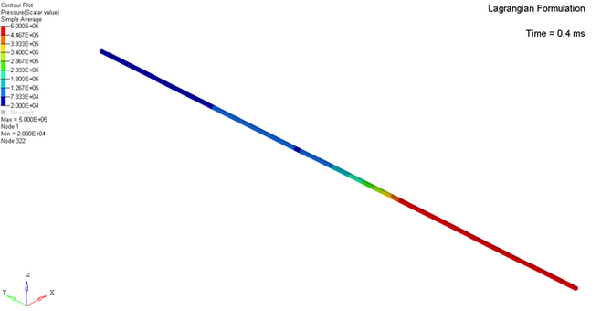
Finite Element Modeling with Lagrangian and Eulerian Formulations
Gas is modeled by 200 ALE bricks with solid property TYPE14 (general solid).
The model consists of regular mesh and elements, the size of which is 5 mm x 5 mm x 5
mm.
Figure 6. Mesh Used for Lagrangian and Eulerian Approaches
In the Lagrangian formulation, the mesh points remain coincident with the material
points and the elements deform with the material. Since element accuracy and time
step degrade with element distortion, the quality of the results decreases in large
deformations.
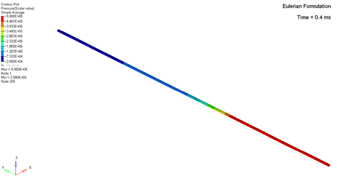
In the Eulerian formulation, the coordinates of the element nodes are fixed. The
nodes remain coincident with special points. Since elements are not changed by the
deformation material, no degradation in accuracy occurs in large deformations.
The Lagrangian approach provides more accurate results than the Eulerian approach,
due to taking into account the solved equations number.
For the ALE boundary conditions (
/ALE/BCS ), constraints are
applied on:
Material velocity
Grid velocity
The nodes on extremities have material velocities fixed in X and Z directions. The
other nodes have material and velocities fixed in X, Y and Z directions.
The ALE materials have to be declared Eulerian or Lagrangian with
/ALE/MAT .