Example 4: Compute the S-Parameters of a Corrugated Horn in the Band from 10 to 20 GHz
This case explains how to calculate S-parameters of a corrugated horn.
Step 1: Create a new MOM Project.
Open newFASANT and select 'File --> New' option.
Figure 1. New Project panel
Step 2: Change the scale to millimeters.

Figure 2. Scale settings
Step 3: Create the geometry of the corrugated horn.
Execute the function “ corrugated_horn(fmin,fmax)” (which can be downloaded). To execute the function, click on Tools - Calculator and write the call to the function.

Figure 3. Calculator panel
- fmin is the lowest operating frequency (GHz)
- fmax is the highest operating frequency (GHz)
The script file, called script_corrugated_horn.nfs, will be automatically generated in the mydatafilesfolder in the newFASANT directory.
The next step is to execute the generated script file. For that, click on Tools – Script - Load and open the script script_corrugated_horn.nfs.
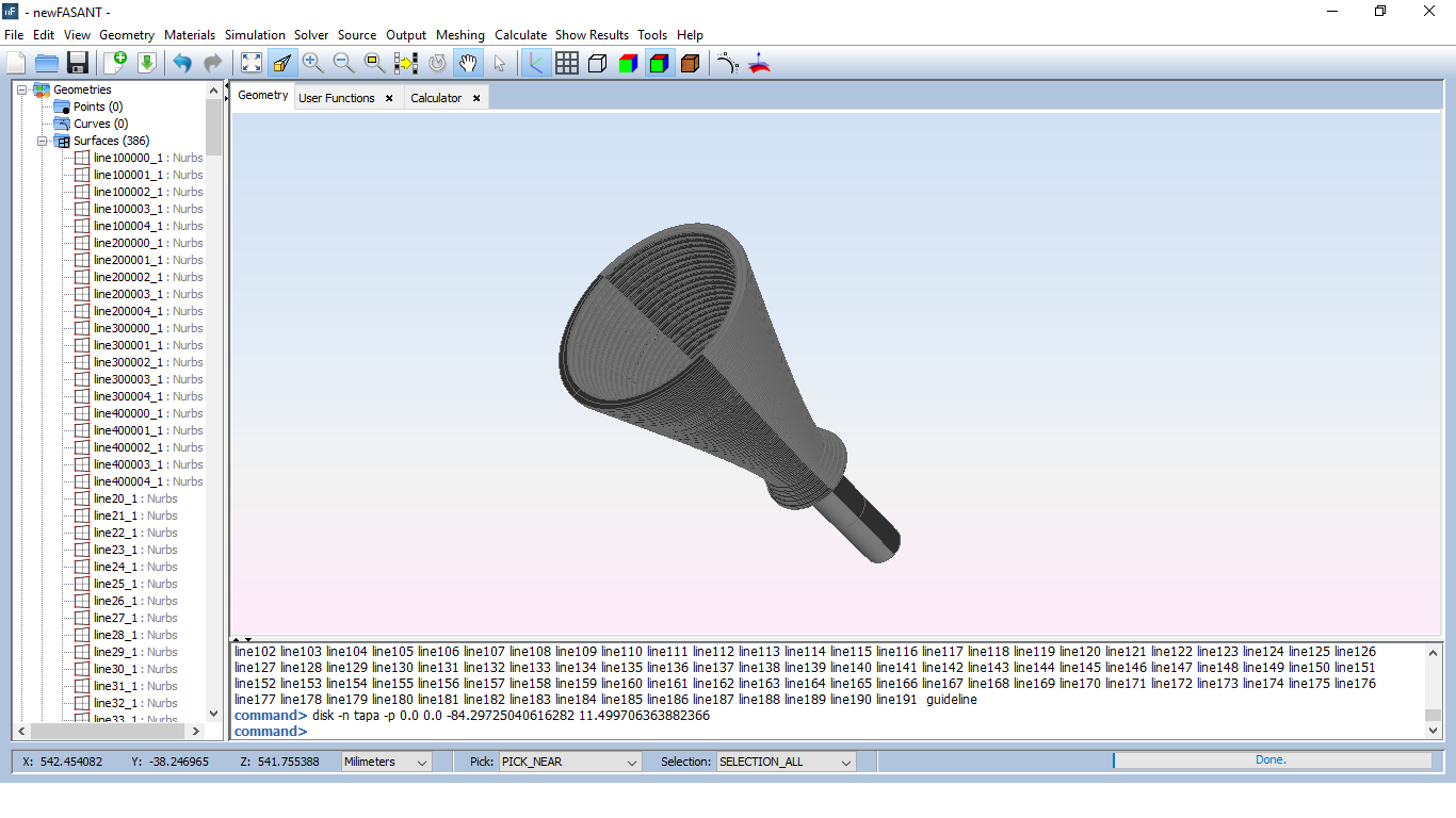
Figure 4. Horn geometry has been generated.
Step 4: Set Simulation Parameters
Select Simulation --> Parameters option on the menu bar and the following panel appears. Set a Frequency Sweep and the S-Parameters Simulation type as shown in the figure below. Remember clicking on Save button to confirm the changes.
Step 5: Set the source parameters.
Note this option requires that the geometry must be only one object (use the group command if it is not) and the waveguide cap needs to be removed
To add a waveguide port, select the object and click on 'Source' --> 'Waveguides' --> 'Add Waveguides Port' menu to open the panel.
And follow the steps described in Add Waveguide Port.
Step 6: Set the solver parameters.
Click on Solver --> Parameters option on the menu bar. Verify that all the parameters are defined by default, as shown in next figure. Click on Save button before going to next step.
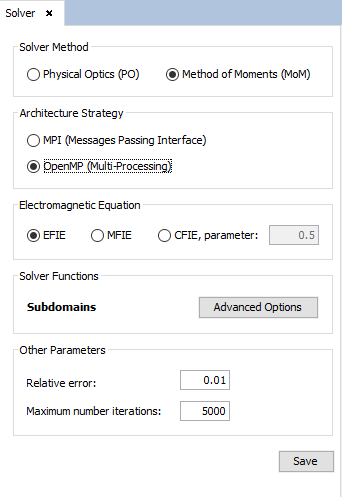
Figure 5. Solver panel
Select ‘Advanced Options’ and activate Preconditioner as shown.
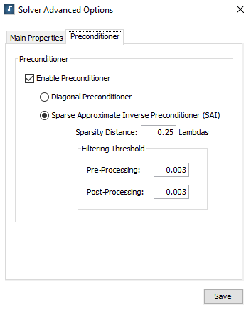
Figure 6. Preconditioner panel
Step 7: Meshing the geometry model.
Select 'Meshing --> Parameters' to open the meshing configuration panel and then set the parameters as show the next figure. In order to obtain the shortest possible time for meshing, it is recommended to run the process of meshing with the number of physical processors available to the machine.
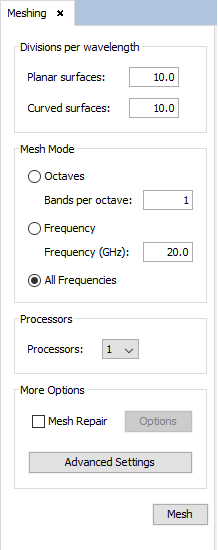
Figure 7. Meshing panel
- octaves: an automatic frequency range per octave is performed, that depends on the Initial and Final frequency. The user can choose 1 frequency by an octave or several frequencies by an octave. The more frequencies per octave, the greater the precision
- all frequencies: a meshing by each frequency is built, so it is the more accurate option. This option will only be chosen when the user needs a very accurate mesh.
Step 8: Execute the simulation.
Select 'Calculate --> Execute' option to open simulation parameters. Then select the number of processors as the next figure show. In order to obtain the shortest possible time for calculating the results, it is recommended to run the process with the number of physical processors available to the machine.
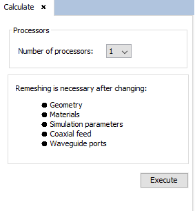
Figure 8. Execute panel
Then click on 'Execute' button to starting the simulation.
Step 9: Show Results.
To get more information about the graphics panel advanced options (clicking on right button of the mouse over the panel) see Annex 1: Graphics Advanced Options.
When the simulation process has finished, the S-Parameters are enabled within the results menu. Click on Show Results menu and S-Parameters option to visualize these parameters. The panel with the available options to visualize the S-Parameters is open on the right side.
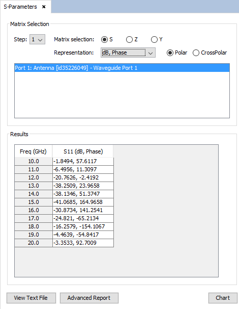
Figure 9. S-Parameters parameters
Select the S-Matrix Representation and the option db, Phase in Representation section. Then, select the column to represent in the Results table and then click on Chart button to add them to plot them.
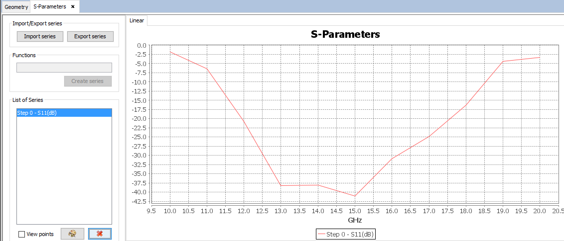
Figure 10. S11parameters plot
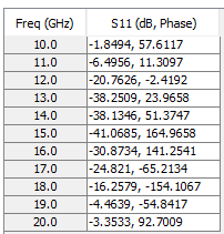
Figure 11. S11 parameters table