SimSolid performs meshless structural
analysis that works on full featured parts and assemblies, is tolerant of
geometric imperfections, and runs in seconds to minutes. In this tutorial,
you will do the following:
Learn how to create bushings for a suspension assembly.
Learn how to change the contact conditions for a specific
subcase.
Solve the modal and transient dynamic subcases and review
results.
Model Description
The following model file is needed for this tutorial:
Bushings.ssp
Figure 1.
This file has the following specifications:
Material is set to Aluminum for all parts.
Regular connections with 0.004mm gap and penetration tolerance.
Modal and Dynamic transient base excitation load subcases are
defined.
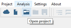
Open Project
Start a new SimSolid session.
Click the (Open Project) icon.
Figure 2.
In the Open project file dialog, choose
Bushings.ssp
Click OK.
Review Connections
On the Connections workbench, click (Find and show disconnected groups of parts).
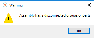
A message appears warning that the model has 2 disconnected groups of
parts. Figure 3. Figure 4.
Click OK.
In the Disconnected groups of parts dialog, review the
groups.
Click Close.
Create Bushing
On the Connections workbench, click > Bushing.
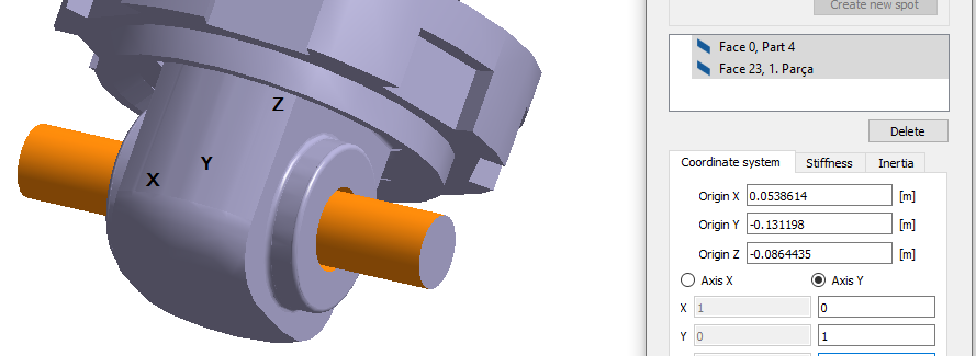
In the modeling window, select the faces as shown in
Figure 5.
Figure 5.
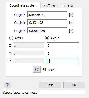
Orient to the global axis.
In the dialog, ensure the Coordinate system tab
is selected.
Select the Axis X radio button and enter
[1,0,0] for X, Y, and Z respectively.
Select the Axis Y radio button and enter
[0,1,0] for X, Y, and Z respectively.
Figure 6.
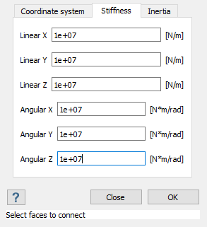
Enter translational-rotational stiffness values.
In the dialog, select the Stiffness tab.
Enter 1e+07 in each text box.
Figure 7.
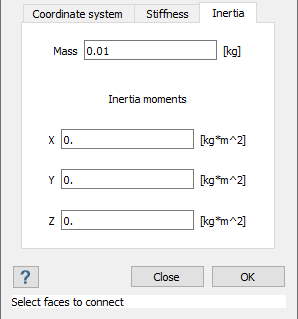
Enter the mass of the bushing.
In the dialog, select the Inertia tab.
For Mass, enter 0.01.
Figure 8.
Click OK.
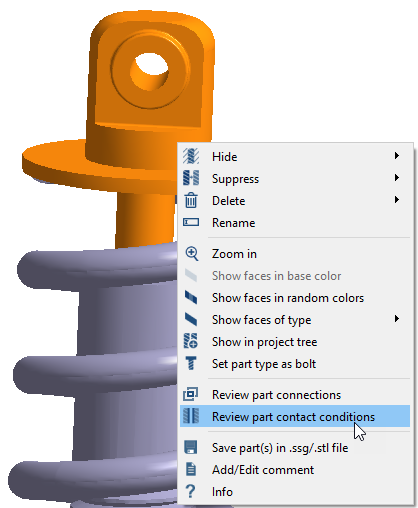
Edit Contact Conditions
In the modeling window, right-click to select the part
shown in Figure 9.
From the context menu, select Review part
contact conditions.
Figure 9.
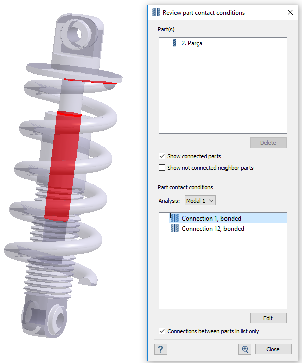
A dialog opens showing contact conditions for all connections associated
with the selected part.
In the Review part contact conditions dialog, select
Connection 1.
Click Edit.
Figure 10.
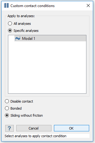
The Custom contact conditions dialog
opens.
Note: Contact conditions can be edited for specific analyses or all
analyses at once. Since there is only one analysis in the design study,
either radio button can be selected.
In the dialog, select the Sliding without friction radio
button.
Figure 11.
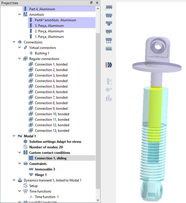
Click OK.
The new contact condition appears in the Project Tree under Modal 1 > Custom contact conditions. Figure 12.
Close all other dialogs.
Run Design Study
Solve all analyses in the design study.
In the Project Tree, click the desired
Design study branch.
Click (Solve).
SimSolid runs all analyses in the design study
branch. When finished, a Results branch for each analysis appears in the
Project Tree.
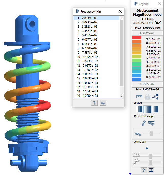
Review Modal Results
In the Project Tree, select the Modal
1 analysis branch.
On the Analysis workbench toolbar, click the
(Results plot) icon.
Select Displacement Magnitude.
The Legend window opens and displays the contour
plot. The Frequency (Hz) window opens and displays the
modes. Figure 13.
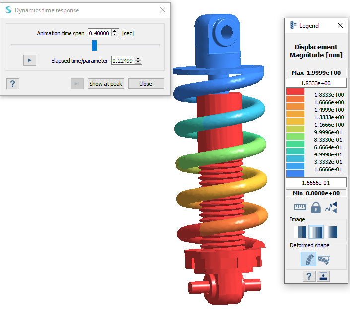
Review Dynamic Transient Results
Plot Displacement Magnitude and von Mises stress.
In the Project Tree, select the Dynamic
transient 1, linked to Modal 1 analysis branch.
On the Analysis workbench toolbar, click the
(Results plot) icon.
Select Displacement Magnitude.
The Legend window opens and displays the contour
plot. The Dynamics time response window opens. Figure 14.
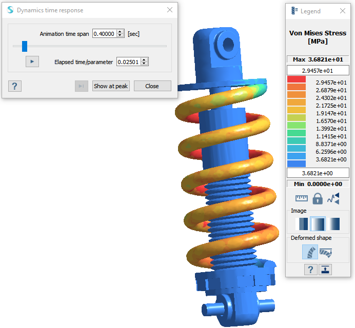
On the Analysis workbench toolbar, click the
(Results plot) icon.
Select Von Mises Stress.
The Legend window opens and displays the contour
plot. The Dynamics time response window opens. Figure 15.
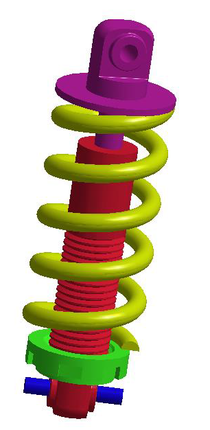 Figure 1.
  (Open Project) icon.
 (Find and show disconnected groups of parts).
A message appears warning that the model has 2 disconnected groups of parts.
(Find and show disconnected groups of parts).
A message appears warning that the model has 2 disconnected groups of parts.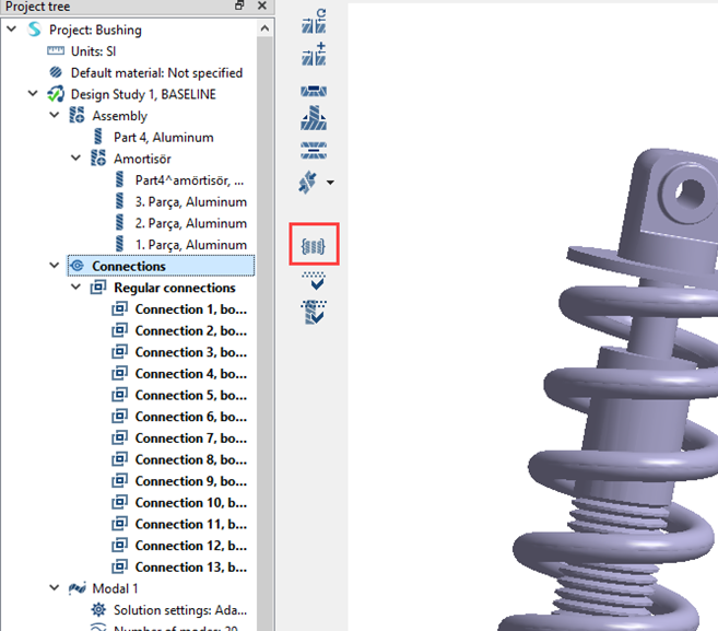
 > Bushing.
 (Solve).
SimSolid runs all analyses in the design study branch. When finished, a Results branch for each analysis appears in the Project Tree.
(Solve).
SimSolid runs all analyses in the design study branch. When finished, a Results branch for each analysis appears in the Project Tree. (Results plot) icon.