PCABLE

Format

<PCABLE
       id       = "integer"
       mid      = "integer"
       area     = "integer"
       iyy      = "integer"
       nx       = "integer"
       nf       = "integer"
       ngx      = "integer"
       ngr      = "integer"
       ngt      = "integer"
       graph    = "integer"
/>

Attributes

id: Unique beam property identification number.
mid: Material property identification number.
area: Element cross section area.
iyy: Element moment of area about y-axis.
nx: Number of integration points in the X direction.; Default for nx is 5.
nf: Number of fibers that the cable is made up of.; Default for nf is 1. 3.
ngx, ngr, ngt: Number of sub elements in X, radial and tangential directions. The default for all three is 1. 4.
graph: A post-processing flag that determines how this element is represented in the animation H3D. Default is 2.

Example

The example demonstrates the definition of a PCABLE property element.

<PCABLE id="1" mid="1" area="78.5398" iyy="490.874" nf="5"  nx="5" ngx="5" />

Comments

This type of property card is used to specify the geometric properties of the CABLE element. Each cable property element must have a unique identification number.
This property card defines the geometrical properties of the cable. The material properties of the beam are defined by the material specified by mid.
A cable is usually made up of multiple wires wound together. For a given cable diameter (D), the bending resistance depends mainly on the number of wires (nf) and the wire diameter (d). Typically, the overall cable diameter (D) is more readily available than the individual wire diameters (d₁, d₂, ..d_n). This is illustrated in the figure below:

Figure 1. A cross section of a cable consisting of multiple wires or fibers

The overall bending stiffness of such a cable decreases as the number of wires or fibers increases. Moreover, this is a non-linear relation. MotionSolve captures this effect by calculating the moment of inertia as:

$I_{y y} = \frac{π}{64 n f} D^{4}$

where

$I_{y y}$

is the calculated element moment of inertia about the y axis

$n f$

is the number of fibers or wires

$D$

is the overall cable diameter

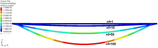
The effect of increasing the number of fibers in the cable element is shown next. A cable component of length 1m is constrained at both ends by a roller support and is allowed to sag due to its own weight. The profile of the cable at steady state is shown for varying value of nf.

Figure 2. The effect of nf on cable element bending stiffness
As can be seen, increasing the number of fibers reduces the bending stiffness of the cable component.
graph is a post-processing flag that determines how this element will be represented in the animation H3D file.
- graph = "0" implies that this element will not be represented in the H3D
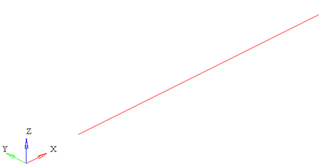
- graph = "1" implies that this element will be represented as a line drawn between the two connecting nodes.
Figure 3. The representation of a cable with graph = 1.

Note: When using graph="0" or graph="1", you will not be able to visualize the stress, strain or displacement contours. To do this, use graph="2" or graph="3".
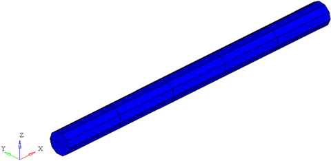
- graph = "2" implies that the cable will be represented by 3D solid elements. This mode is useful when trying to visualize the stress/strain and displacement contours.
Figure 4. The representation of a cable with graph = 2. The cable is represented by 3D elements
- graph = "3" implies that the cable is represented both as 3D solid elements as well as a line connecting the two nodes of the cable. This is useful when you need to visualize both the center line and the 3D representation of the cable.
Figure 5. The representation of a cable with graph = 3. The 3d elements in the middle of the cable are turned off to show the center line of the cable

When representing the cable as a solid, the arguments ngx, ngr and ngt determine the number of elements that are used to represent the cable in the animation H3D.

Figure 6. Effect of ngx, ngr and ngt on the 3D representation of a simple cable

ngx = ngr = 1; ngt = 1

ngx = ngy = 2; ngt = 12

While increasing the ngx, ngy and ngz results in a better representation of the cable, it also increases the post-processing time taken by MotionSolve to write out the H3D. In addition, large values of ngx, ngy and ngz will increase the file size of the H3D considerably. Consider using the minimum values of these attributes that satisfy your visualization needs.