Magneto-thermal coupling: general information
Studied devices
The magneto-thermal co-simulation is meant for electric devices such as motors, transformers or busbars.
Applications: Magnetic
In magnetic 2D/3D magnetic Flux, the magneto-thermal coupling is usable for the following
applications:
- Transient magnetic, with the following two options:
- To export the average value over a period of the calculated losses, in case of the study on the motor steady state regime, or
- To export the instantaneous value of losses, in the case of the study on the motor start-up
- Steady state AC magnetic
In Flux PEEC, an application dedicated to the co-simulation exist :
“Supplied conductors with thermal coupling”. It corresponds to a steady state AC magnetic application defined by one or several frequencies.
Applications: thermal
In 2D/3D thermal Flux, the magneto-thermal coupling is usable for the following
applications:
- Steady state thermal
- Transient thermal
In STAR-CCM+, the concerned applications are:
- Steady state thermal
Solution brought about by Flux
The magneto-thermal coupling is accessible via the multiphysic context of Flux, and is named in Flux: « cosimulations ».
New entities/boxes are present in this context in order to manage the
«cosimulations». Example: «exported data», «imported data» etc.
Once the cosimulation entities have been defined, the communication between the two pieces of software (Flux-Flux or Flux coupled to another software) is automatically controlled via the synchronization files for postponing or launching the calculation.
This new mechanism replaces the editing of python scripts which formerly had to be written for each simulation.
New entities dedicated to the cosimulation in Flux:
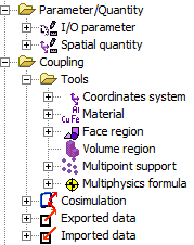
Environment
Once the geometry, mesh and physics have been defined and the solving scenario has been created, the multiphysics context is accessible through the menu .
Solution brought about by STAR-CCM+
With STAR-CCM+, an interface presented as a Wizard named «Simulation Assistant» has been constructed in order to guide the user in the introduction of the cosimulation data. The input windows are equivalent to those in Flux.
Automatic synchronization of actions
The synchronization between the two software programs is carried out by files:
- The software application that is working generates a postponing file for the other software
- When it makes a data export, an authorization file for the start of the third party software computation is generated
- Once the convergence has been attained, a file for the stop of the iterative computation is generated
- When the solving process is over, or if a problem occurs during this process, then a stop file is generated.
Data computed and exported in Flux
Starting from 2D/3D Flux electromagnetic project, the volume density of the losses is exported:
- Joule losses: the formula dLossV is exported, in W/m3 on each node
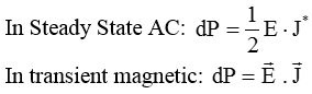
- Bertotti or LS iron losses : in W/m3* on each node
In a Flux PEEC project, volume density of Joule losses in W/m3 are computed and exported
In Flux, the values of the losses volume density vary from a cosimulation step to step because materials properties are temperature dependant and the temperature is updated after each thermal computing step. Example :
![]() or
or ![]()
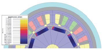 Figure 1. Magnet losses
Data computed and exported in the thermal software
In the thermal software are exported :
- The temperatures in Kelvin at each node
In the thermal software, the temperature field vary from a co-simulation step to step because the heat sources (equal to losses) are updated after each electromagnetic computation.
Main steps
In the table below, the main steps to follow in Flux electromagnetic are described for the cosimulation setting up (in Flux thermal the steps are similar).
| Step | Action |
|---|---|
| 0 | Create the project and define the physics taking into consideration the temperature dependence of the materials properties |
| 1 | Open the multiphysics context by a solving scenario |
| 2 | Export the nodes of the electromagnetic regions on which the thermal calculation will be carried out |
| 3 | Create «multipoint supports» starting from the files of nodes coordinates of the thermal software |
| 4 | Create «multiphysics formulas» that comprise the formulas of the quantities to export (Joule Losses, iron Losses …) |
| 5 | Create «data to export» that define the multiphysics formula, the multipoints calculation support etc. |
| 6 | Create «data to import» that define the spatial quantity and the region receiving the imported values etc. |
| 7 | Create the «cosimulation » defining the type of cosimulation, the convergence accuracy, the data to export and to import etc. |
| 8 | Solve the cosimulation |