Steps of thermal project description in STAR-CCM+
Presentation
Step 0 : prepare the projet
Prepare the project (geometry, mesh, physics).
For the moment, only steady state thermal application works in the cosimulation.
The step 1 can be started once the first non-zero losses values are exported from Flux (verify that the exchange directory contains the “Starccm_run.sync” file)
Step 1: Open the Wizard
A wizard is available and it guides the user in the cosimulation data preparation.
To open the wizard, user has to load the file « Flux-STAR-CCM__Co-Simulation.jar ».
The wizard is available through the menu or through the icon ![]()
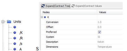
Step 2 : verify the units
Verify the project units, as for example the temperature units:
Step 3 : Identify exchanged data names
Given that the cosimulation communication is done with files, in STAR-CCM+ the files names (chosen in Flux) have to be recognized. For that, the « STARCCM_INIT.SYNC » file has to be loaded (the file is generated by Flux automatically after the cosimulation entity creation).
After that, the imported and exported data list is visible in the data tree, in Tools/Tables.
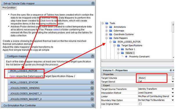
Step 4 : Define the imported data
The imported data (heating sources) have to be associated to thermal regions.
For that, you should :
- First, click on the first link presented below. The « configure mappers » will be filled with imported data list,
- Then click on « open » of each imported data. The associated zone in the data tree will be opened,
- And finally the right volume has to be chosen to store the heating source values.
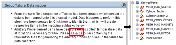
Step 5: create the multipoints supports
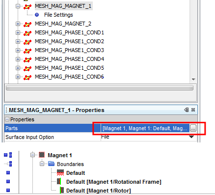
Then the equivalent of multipoints supports (name in Flux) called « Derived Parts » in STAR-CCM+ have to be created with the magnetic mesh.
For that you have to :
- Click on the link below
- Choose the mesh .VTK files (it is enough to select only the first file; all the others will be automatically managed). All the derived parts are created then.
- Associate for each derived part the corresponding region by clicking on the button as below (select the regions with the “boundaries”)
Remark: in the case of 2D Flux project, the 2D Flux mesh contained in the derived parts is placed on the 2D centred plane (in z).The computation & export will be done on this plane mesh.
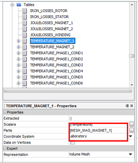
Step 6: associate the supports and the quantity to the exported data
The Derived parts are automatically associated to the exported data if the names extensions after the last « _ » are the same. If it is not the case, the association has to be done manually in the exported data.
The exported quantity “Temperature” has to be chosen in the corresponding field.
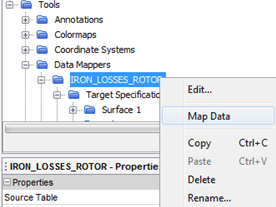
Step 7 : Create the mapped heat sources
Create the heat sources mapped on STAR-CCM+ mesh from the heat losses computed on Flux mesh. For that:
Create “scalar field functions” corresponding to the heat losses for each data mapper mapped on STAR-CCM+ mesh :
Automatically the following « field functions » are created :
![]()
Remark: in case of 2D Flux project, the losses volume densities are mapped on the centered 2D plane mesh in STAR-CCM+, and then repeated in the depth (in z) in the corresponding region.
Step 8 (optionnal) : adjust interpolation
Depending on the cases, an adjustment can be done on the losses computed on STAR-CCM+ mesh, because the integral value doesn't correspond exactly to the losses integral computed on Flux mesh.
To create the adjusted mapped values:
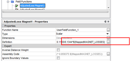
1) Create new scalar Field functions manually:
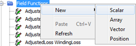
2) Rename the scalar function and define it by multiplying the previous « mapped LOSSES » with the ratio : Flux losses integral / Interpolated losses integral :
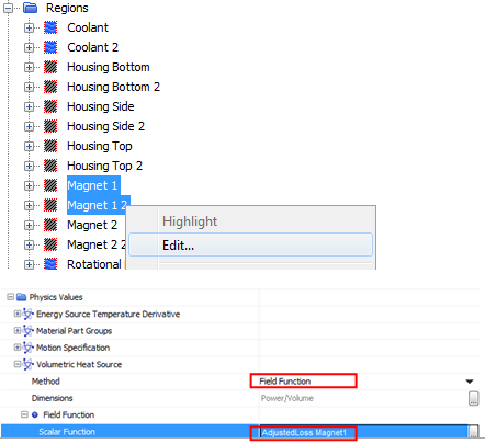
Step 9 : losses assigning into regions
The adjusted losses (or interpolated losses without adjustment) have to be assigned to the corresponding regions :
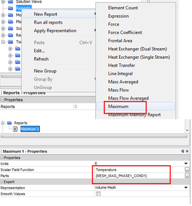
Step 10 : stopping criteria definition (1)
In STAR-CCM+, a stopping criteria has to be defined to stop the STAR-CCM+ simulation and hand over to Flux.
For example, the STAR-CCM+ solving can stop when the maximum temperature in the winding varies less than 1K during 10 iterations.
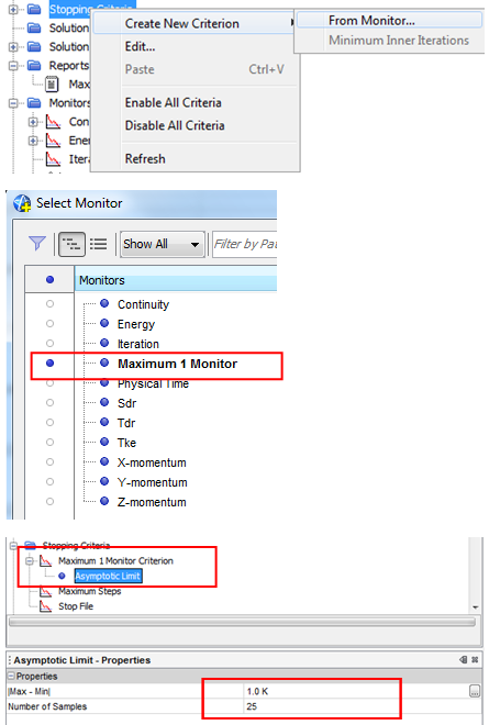
1) create a new report corresponding to a “Maximum” of the temperature in the winding
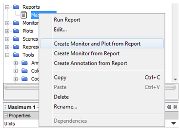
2) Create a Monitor from the previous Report to create after a stopping criteria and to open the maximum temperature curve depending on the iterations:
3) Create the stopping Criteria from the previous monitor and choose “asymptotic limit” criteria defined by a variation lower than 1K during 10 iterations :
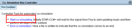
Step 11 : Launch the cosimulation
The last step is to launch the cosimulation on STAR-CCM+ side:
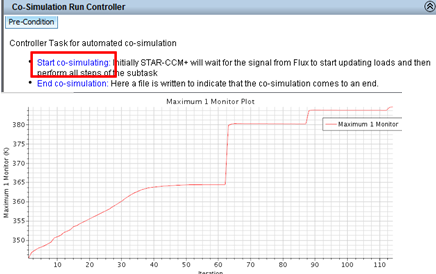
Step 12 : stop the cosimulation
It is possible for the user to enter a cosimulation convergence criterion in Flux, what will stop automatically the cosimulation.
If the user has not entered this criterion in Flux, he has to look in STAR-CCM+ at the chosen curve and stop manually the cosimulation when it has converged as he expected. (The curve contains all the temperature results from the beginning of the cosimulation).
To stop the cosimulation click on “End cosimulation”:
Remark
If the user has launched a cosimulation, closed the STAR-CCM+ file, then after opening the simulation file it is possible to launch again a cosimulation by following the steps :- Load once again the « starccm_init.sync » file
- Delete the duplicated « data mappers » and then the « table » entities (with the « _2 » extension)
- Delete the old results by clicking on the command : « clear solution » in the « solution » menu