Application example

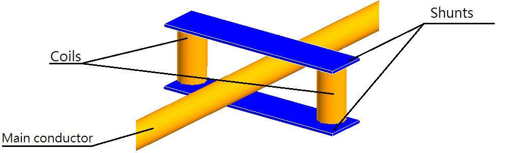
This example shows the advantages of the integral method compared to the conventional finite element approach for a current sensor. In this case, a current is injected into the main conductor and we are looking to compute the magnetic flux observed by the auxiliary coils, as shown in Figure 1. The characterization of this sensor requires knowledge of its gain and crosstalk.

Figure 1. Full device

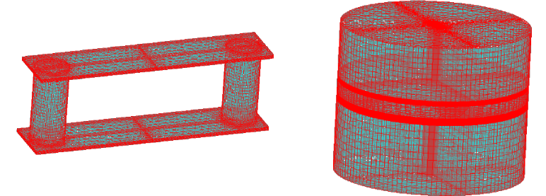
This device being characterized by a large quantity of leakage flux and by the distances between the conductors that can be large, the use of the conventional finite element method requires to intensively mesh the surrounding air. To get results approaching the real the solution, the mesh must be symmetrical and very dense, which increases the computation time (see Figure 2).

Figure 2. On the left, the mesh of the device. On the right the mesh of the air.

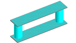
The integral method is much cheaper in terms of meshing elements because we do not mesh the air anymore (see Figure 3).

Figure 3. Mesh for the integral method

Comparison of the two methods: For the computation of the flux in a coil, the volume integral method is also faster than the finite element method. This magnetic flux is split into two contributions, the contribution of the other coils and the contribution of the magnetic parts [2]. In the air and for the other coils we compute the magnetic flux by a Biot & Savart law. For the magnetic parts the computation is done with the magnetic vector potential already computed in resolution.

The study of this sensor requires to know its gain defined in the frequency domain by the following relation: $G_0= \frac{2\pi \phi f}{I_0}$ with

• f : the frequency
• $I_0$ : the current in the main conductor
• $\phi$ : the magnetic flux in the auxiliary coils

We can compute the gain for several values of current :

Figure 4. Gain of the sensor

Figure 4 shows that the finer the mesh is, the more the results will be close to the real solution and therefore to the solution provided by the integral method.

A complete study also requires knowing the crosstalk of the sensor, $\lambda = \left|\frac{G}{G_0}\right|$ with,

• G : the gain corresponding to the sensor with an offset on the position of the main conductor.

Figure 5. Crosstalk of the sensor