Post-processing quantities
Introduction
The post-processing quantities are of two types:
- local quantities, analyzed in all points of the study domain,
- global quantities*, resulting from an integration, analyzed over the entire study domain or on a part of this domain.
Note: * In the presence of symmetries and/or periodicities these quantities are computed
for the part of the device represented in the finite elements domain.
Usual quantities
Usual local quantities available are presented on the table below.
| Usual quantities |
Flux formula |
Flux Unit | Explanation | Application | ||
|---|---|---|---|---|---|---|
| 2D plane | 2D axi | 3D | ||||
| Temperature | Temp(Tkelvin) | K |
|
|
|
|
| Temperature (gradient) | mGradT | K/m |
|
|
|
|
| Heat capacity (volume): ρCP | RhoCp | J/(m3 .K) |
|
|
|
|
| Thermal conductivity: k | Kth | W/(m.K) |
|
|
|
|
| Thermal flux (surface density): |
dFluxTh | W/m2 |
or
|
|
|
|
Advanced use
Usual local quantities available in advanced use are presented on the table below.
|
Quantities (advanced use) |
Flux formula | Flux Unit | Explanation | Application | ||
|---|---|---|---|---|---|---|
| 2D plane | 2D axi | 3D | ||||
| Temperature (Kelvin): TKelvin | TKelvin | K |
|
|
|
|
| Temperature (Celsius): TCelsius | TCelsius | °C | TCelsius = TKelvin -273.15 |
|
|
|
| Heat (volume density): q | dHeatV | W/m3 |
|
|
|
|
| Heat (surface density): q | dHeatS | W/m2 |
|
|
|
|
| Heat (line density): q | dHeatL | W/m |
|
|
|
|
| Heat transfer (convection coefficient): h | Hconv | W/(m2.K) |
|
|
|
|
| Hconv2s | (on both sides, for regions with double heat exchange) | |||||
| Heat transfer (radiation coefficient): ε | Hrad | W/(m2 .K4) |
|
|
|
|
| Hrad2s | (on both sides, for regions with double heat exchange) | |||||
|
Ambiante temperature (for convectif exchange) |
Tamb | K |
|
|
|
|
| Tamb2s | (on both sides, for regions with double heat exchange) | |||||
| Heat transfer (surface density): |
dExchangeS | W/m2 | 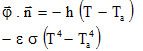 * * |
|
|
|
Note: * If the local radiation is applied, the second term is to replace by the thermal
flux expression given in the part 1.1.6 of this document.
Global quantities
Global quantities are not directly available. They can be calculated by integration (See § Explanation of results)