Adjusting parameters in the Newton-Raphson method

Adjusting parameters

Newton-Raphson parameters and strategies are set automatically to ensure robustness and fast non-linear solving. It is nevertheless possible for the user to adjust these parameters, using the Nonlinear system solvers tab of the Solving process options box.

Adjusting of Newton-Raphson method

The user can adjust the following Newton-Raphson parameters :

Type of accuracy threshold : Global based or variable based convergence. Except for 2D and 3D hysteresis projects, for the optimal with stabilization stage relaxation method and with 2D initialization for Skew, in which we observed better performances and robustness with global convergence, variable based convergence is set automatically. It ensures that all the variables of the system satisfy the required precision, where global convergence relies on the variable with the most difficult convergence.
The threshold: Relative epsilon value below which Newton-Raphson non-linear solver stops. Depending on the activation of looseness and/or strengthening, this threshold is fixed or is the starting point of the adaptive criteria strategy. Default value is 10e^-4.
Maximum number of Newton-Raphson iterations. The default value is 100.

Adaptive criteria strategy relies on hard or easy convergence detection

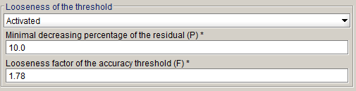
Figure 1. Easy (yellow), normal (green) and hard (red) convergence illustration
Losseness of the threshold : This adaptive criteria strategy is meant to ease hard convergence. The adaptation is based on the residual decrease between two consecutive Newton-Raphson iterations.
If the decrease between these two residuals is less than a percentage P (default is 10%), we consider a hard convergence situation (Red region on Figure 1). If we have a hard convergence situation, the threshold is multiplied by a factor F (default is 1.78) to ease the convergence.
Percentage P and factor F can be modified in advanced mode:

This strategy is activated by default, except for 2D and 3D hysteresis projects, for the optimal with stabilization stage relaxation method for non-linear project and 2D initialization strategy for Skew.
Strengthening of the threshold : This adaptive criteria strategy is meant to harden easy convergence. The adaptation is based on the residual decrease between two consecutive Newton-Raphson iterations.
If the decrease between these two residuals is more than a percentage P (default is 99%), we consider a too easy convergence situation (Yellow region on Figure 1). If we have too easy convergence situation, the threshold is divided by a factor F (default is 3.16) to harden the convergence.
Percentage P and factor F can be modified in advanced mode:

This strategy is activated by default, except for 2D and 3D hysteresis projects, for the optimal with stabilization stage relaxation method for non-linear project and 2D initialization strategy for Skew.

Under-relaxation method (3D)

There are five methods for defining the relaxation coefficient a of the Newton-Raphson method:

the stairs method, where the coefficient is determined at each Newton-Raphson iteration, according to a simple law that depends on the obtained accuracy by the Newton-Raphson algorithm,
the fixed method, where the user inserts the coefficient value which is thus constant throughout the solving process,
the optimal method, where the coefficient is determined at each Newton-Raphson iteration by minimizing the residual of the nonlinear system to be solved,
the automatic method, where the program automatically determines, depending on the formulation, which method is used, the "stairs" or the "optimal" one.
The maximal factor method, which computes at each Newton-Raphson iteration the largest coefficient such that the residual of the non-linear system to be solved decreases.

The automatic method is the method chosen by default. These four methods are detailed in the following paragraph.

Stairs method

The relaxation coefficient is determined at each Newton-Raphson iteration, function of the value of the precision ε^i-1 obtained at the previous iteration, following the variation law given below:

at the first iteration:

α = 0,5
at the next iterations:
- si ε^i-1 ∈ [0,1 ; +∞[ : α = 0,5
- si ε^i-1 ∈ [0,01 ; 0,1[ : α = 0,75
- si ε^i-1 ∈ [0 ; 0,01[ : α = 1

Fixed method

The value of the relaxation coefficient is inserted by the user in the interval ]0 ; 1]. The value of this coefficient is thus constant throughout the solving process.

Optimal method

The relaxation coefficient is determined at each iteration. The principle of the method consists of computing this coefficient so that the following objective function is minimum:

W^{i} = \sum_{j = 1}^{n} {(R_{j}^{i})}^{2}

where $R_{j}^{i}$ is the j-th component of the residual R(Xⁱ) at the i-th current Newton-Raphson iteration (R(Xⁱ) is a vector with n elements). n is the number of unknowns of the system.

The search of the objective function minimum is carried out using an iterative method, due to the fact that W cannot be explicitly expressed function of α. The search is performed by computing the values of Wⁱ for the values of

α = α_k = 1/2^k-1 (α = 1 then 1/2, 1/4, 1/8...), and it is stopped when Wⁱ_k+1 at the iteration k+1 is greater than Wⁱ_k at the previous iteration k. Indeed, during the iterations, α = α_k = 1/2^k-1 decreases and Wⁱ_k decreases up to a certain iteration and then it increases.

Automatic method

Flux 3D automatically determines function of the formulations used for the regions, which is the best relaxation method.

Flux 3D automatically chooses the stairs relaxation method, except for the regions that use a non-surface impedance formulation in magnetic scalar potential (reduced or total), for which the optimal method will be used. The automatic method is the default method.

Maximal factor method

The relaxation coefficient (α) is computed at each Newton-Raphson iteration. This method consists in searching the largest coefficient satisfying a decrease of the residual of the non-linear system. To do that, the residual is computed with different values of α, by first trying to increase this coefficient (maximum to 1) before decrease it only if the residual of the non-linear system did not decrease with respect to the previous Newton-Raphson iteration.

More in details, the strategy is the following: at the i^th Newton-Raphson iteration, the algorithm starts with the relaxation coefficient α of the previous Newton-Raphson iteration (α=1 at the first iteration). Then it first increases that coefficient (α = min(αφ,1), with φ the golden ratio) and computes the new residual of the non-linear system.

If that residual is less than the residual of the previous Newton-Raphson iteration, the algorithm continues to increase that coefficient with the same rule, until it reaches α = 1 or obtains a residual greater than the one of the previous Newton-Raphson iteration. It will then keep the last α (the largest) which decreases the residual.
If this residual is greater than the residual of the previous Newton-Raphson iteration, the algorithm decreases that coefficient (α = max(α/φ,β), with β the minimum relaxation coefficient, depending on the project and defined by Flux). If the residual becomes less than the one of the previous Newton-Raphson iteration then the algorithm keeps that coefficient, else it continues to decrease the coefficient, following the same rule.