Solving a nonlinear system: Newton-Raphson method
Nonlinear system: matrix form equation
A nonlinear system (n equations and n unknowns) can be written under the form:
[A(X)].[X] = [B] (Equation 1)
where the system matrix A depends on the vector solution X.
Nonlinear system: solving
The solution of a nonlinear system is obtained by using an iterative procedure, i.e. by solving a set of linear systems, the solutions of which are convergent towards the solution of the nonlinear system.
There are different techniques of solving nonlinear systems, but the convergence of the solving process is never guaranteed. The method used in Flux is the Newton-Raphson (NR) one. This method is applied to equations of the form f(x) = 0 for which the derivative f'(x) of the function f can be computed.
The NR method is briefly presented in the following paragraphs:
- through a “numerical approach”
- through a “graphic approach” on an example
NR Method: numerical approach
Introducing the vector matrix function: [R(X)] = [A(X)].[X] - [B]
the equation 1 can be written under the form: [R(X)] = 0
The NR method allows the evaluation by an iterative method of the zero of function R(X) starting from the Taylor series formula.
The matrix equation to be solved is written under the form:
![]()
where:
- dR/dX matrix is the Jacobian of the system
- R(X) is the residual vector
An increment ΔX of the solution is computed at each step
The vector solution is written:
![]()
The process stops once the criteria εi < ε is reached, where:
- εi = ||ΔXi+1||/||Xi+1||.
- ε is the precision of the Newton-Raphson procedure, provided by the user
NR Method: Graphic approach (1)
The Newton-Raphson method, also known as the tangent method, is presented now through a “graphic approach”, on an example, in the figure below.
Example (Magneto Static application):
The differential equation solved using finite element method in a magneto static application (with the vector model) is written under the following form:
![]() (Equation 2)
(Equation 2)
where:
- ν is the magnetic reluctivity of the isotropic computation domain
 is the density of current source
 is the vector potential, respectively the state variable,
i.e. the unknown of the system.
is the vector potential, respectively the state variable,
i.e. the unknown of the system.
Hypothesis:
We can say that solving equation 2 is the equivalent of finding the value B for H = Hs on the characteristic B(H). Hs is the magnetic field generated by the current source Js.
Graphic approach of the method:
We “arbitrarily” choose a first value of the unknown B, zero for example, and we replace the curve by its tangent. Afterwards, we can easily compute, by using the equation of the tangent (a line equation), a second value of B and continue with the second iteration. By successive iterations, a value of B ever closer to the required value of B is obtained.
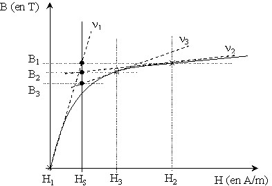
-
1st iteration (at the origin): B = 0 tangent of ν1 slope
computation of B value associated to the tangent (B when H = Hs) ⇒ B1
-
2nd iteration: B = B1 tangent of ν2 slope
computation of B value associated to the tangent (B when H = Hs) ⇒ B2
-
3rd iteration: B = B2 tangent of ν3 slope
computation of B value associated to the tangent (B when H = Hs) ⇒ B3 …