ACU-T: 1000 HyperWorks UI Introduction
This tutorial provides the instructions for setting up a Computational Fluid Dynamics (CFD) simulation making use of the HyperWorks package. HyperWorks is a comprehensive suite of various Computer-Aided Engineering (CAE) products, each specialized in a certain aspect of the CAE process. These include HyperMesh as a generic, powerful geometric modeling and pre-processing tool, and HyperView as a post-processing and visualization tool. Bridging these two applications is a complete range of solvers for a gamut of engineering applications. Among these solvers is AcuSolve, which is Altair’s offering for fluid flow and thermal analysis simulations.
HyperMesh’s inbuilt geometric modeling and finite element meshing capabilities will allow you to create the geometry for your problem and generate excellent quality meshes in a single tool. Meshes generated in HyperMesh can be exported in the format that AcuSolve will recognize. Moreover, HyperMesh’s integration with AcuSolve also allows you to complete the pre-processing steps in HyperMesh itself, including the problem setup. Once you have completed setting up your simulation in HyperMesh, you can directly generate the AcuSolve input files. You can also choose to directly launch AcuSolve from within HyperMesh. This integration is expected to be especially beneficial for you if you happen to be a traditional user of HyperMesh for your modeling and meshing requirements.
The HyperWorks package has a powerful tool for post-processing and visualizing the results of your CFD simulations, called HyperView. HyperView enables you to visualize data interactively as well as capture and standardize your post-processing activities using process automation features. HyperView combines advanced animation and XY plotting features with window synching to enhance results visualization. HyperView also saves 3D animation results in Altair's compact H3D format so you can visualize and share CAE results within a 3D web environment using HyperView Player. HyperView has a rich feature set that you might find beneficial to your post-processing activities and are useful to explore. HyperView has inbuilt direct-reading capabilities for AcuSolve results and does not require any conversion steps.
In this tutorial, you will learn how to use HyperMesh for importing a geometric model and generating a mesh. You will then set up and launch the simulation from within HyperMesh. Following that, you will learn how to use HyperView for post-processing AcuSolve results.
- Analyze the problem
- Start HyperMesh and create a model database
- Import the geometry for the simulation
- Generate and organize the mesh using the Mesh Controls Browser
- Set general problem parameters
- Set solution strategy parameters
- Set the appropriate boundary conditions
- Run AcuSolve
- Monitor the solution with AcuProbe
- Post-process with HyperView
Prerequisites
To run this simulation, you will need access to a licensed version of HyperMesh and AcuSolve. This tutorial introduces you to HyperMesh and HyperView so no prior experience is expected.
Prior to running through this tutorial, click here to download the tutorial models. Extract ACU-T1000_manifold.x_t from HyperMesh_tutorial_inputs.zip.
The file ACU-T1000_manifold.x_t stores the geometry information for the fluid portion of the model for this problem in Parasolid ASCII format.
The color of objects shown in the modeling window in this tutorial and those displayed on your screen may differ. The default color scheme in HyperMesh is "random," in which colors are randomly assigned to groups as they are created. In addition, this tutorial was developed on Windows. If you are running this tutorial on a different operating system, you may notice a slight difference between the images displayed on your screen and the images shown in the tutorial.
Analyze the Problem
An important step in any CFD simulation is to examine the engineering problem at hand and determine the important parameters that need to be provided to AcuSolve. Parameters can be based on geometrical elements, such as inlets, outlets, or walls, and on flow conditions, such as fluid properties, velocity, or whether the flow should be modeled as turbulent or as laminar.

Figure 1. Schematic of the Problem
Introduction to HyperMesh
HyperMesh is a generic tool offering a combination of geometric modeling and pre-processing capabilities.
HyperMesh supports a number of commonly used solvers used in simulating various engineering applications, providing direct interfaces to most of them. This offers you flexibility to use HyperMesh as a single tool for most, if not all, of your modeling and pre-processing activities.
AcuSolve is among the solvers that are closely integrated with HyperMesh. In order to simplify the interfaces associated with each solver, HyperMesh uses user profiles to automatically manage the templates for a given solver. Each user profile has an associated pre-defined set of menus, options and toolbars visible. User profiles ensure that the solver setup is in accordance with the options and requirements of the solver associated with the profile in which it is generated. It is advised that you make sure you are using the correct user profile when setting up a model. Also, it is recommended that the active user profile is not to be changed while the current HyperMesh database is populated.
In this tutorial, you will be working in a user profile associated with AcuSolve. Once you begin the tutorial, you will change the active user profile to the AcuSolve user profile. HyperMesh remembers the last active user profile when it is restarted. If the last HyperMesh user on your machine was working in the AcuSolve user profile when you launch HyperMesh, it will start with the AcuSolve user profile.
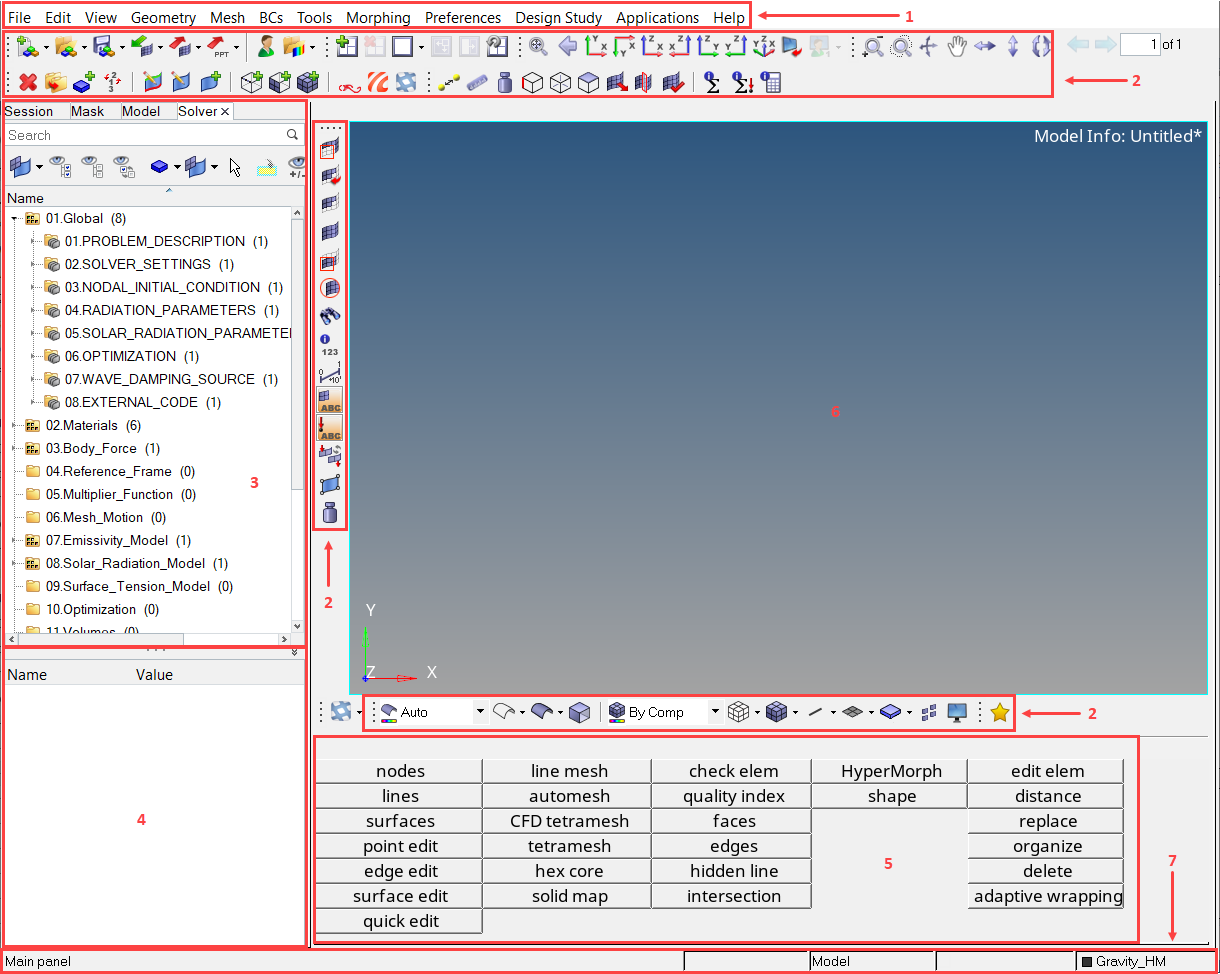
Figure 2. HyperMesh Interface with Active AcuSolve User Profile
- Menu bar: Located at the top of the window, just under the title bar. Like the pull-down menus in many applications, these menus drop-down a list of options when clicked.
- Toolbars: Located around the modeling window. These have icons
that provide quick access to commonly-used functions, such as changing display options.
They can be dragged and placed as per the user preference. Below are some of the commonly used toolbars.

Figure 3. Standard ToolbarProvides the options for creating, opening or saving the database, import/export options and changing user profiles.

Figure 4. Checks ToolbarOn the Checks toolbar, you can access various checks and calculations tools that are commonly used in the model building process.

Figure 5. ACU ToolbarThe ACU toolbar has options for creating, deleting and organizing entities, accessing meshing panels, and launching AcuSolve or HyperStudy.

Figure 6. Display ToolbarOn the Display toolbar, you can control what entities HyperMesh displays, primarily by masking entities to hide or display. This toolbar is usually located along the left edge of the modeling window.

Figure 7. Visualization ToolbarOptions available on the Visualization toolbar control how HyperMesh visualizes entities in the modeling window.
- Tab area: The two areas marked 3 and 4 in Figure 2 make up the tab area. The tab area is so named because various specialized tools display on tabs in this area of the interface. One of these tabs is the Model tab, which you will be using most frequently. The Model tab will also be the tab active by default when you start a HyperMesh session. The top half of the tab area, marked 3, is the browser area. Depending on the selected tab, you will be able to see the various options or entities which belong to the active HyperMesh database. For example, when the Model tab is selected, the Model Browser will display the entities present in the model, each of which carry some information about the model. This information may be related to the geometrical components that make up the model, the material information, the load information, and so on. The model structure is viewed as a flat, listed tree structure within the browser.
- Entity Editor: The bottom half, marked 4 in Figure 2, is the Entity Editor. In the Entity Editor, you will be able to view and edit the information associated with the different entities available in the browser. Clicking on an entity in the browser area will display the entity related information in this area.
- Main Menu: The main menu displays the available functions. You access these functions by clicking on the button corresponding to the function you want to use. Clicking on the button will open the panel associated with the function in the menu area.
- Modeling Window: The modeling window is the display area for your model. You can interact with the model in three-dimensional space in real time. In addition to viewing the model, entities can be selected interactively from the modeling window.
- Status bar: The status bar is located at the bottom of the screen. The four fields on the right side of the status bar display the current include file, current part, current component collector and current load collector. As you work in HyperMesh, any warning or error messages also display in the status bar on the left side.
Introduction to HyperView
HyperView is a generic post-processing and visualization environment for finite element analysis (FEA), CFD, multi-body system simulation, digital video and engineering data.
HyperView offers direct-reading capabilities for AcuSolve generated results. AcuSolve results can be directly opened in HyperView. HyperView also has process automation features, which can enable you to expedite and standardize your post-processing activities.
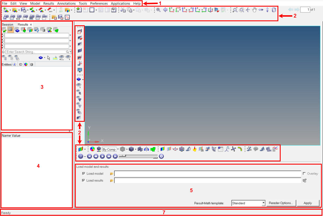
Figure 8. HyperView
- Menu bar: Located at the top of the window, just under the title bar. Like the pull-down menus in many applications, these menus drop-down a list of options when clicked.
- Toolbars: Located around the modeling window. These have icons
that provide quick access to commonly-used functions, such as changing display options.
They can be dragged and placed as per the user preference. Below are some of the
commonly used toolbars.
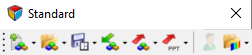
Figure 9. Standard ToolbarProvides the options for creating or opening a model, saving an HyperView session and import/export options.
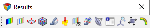
Figure 10. Results ToolbarOn the Results toolbar you can access various options related to displaying the results, for example, contours, vectors and streamlines.
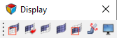
Figure 11. Display ToolbarThe Display toolbar provides you with quick access to the Mask panel, Section Cut panel and Display Controls.
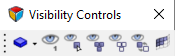
Figure 12. Visibility Controls ToolbarThe Visibility Controls toolbar provides you quick access to the visibility controls of the entities in the Results Browser.
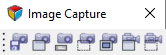
Figure 13. Image Capture ToolbarThe Image Capture toolbar provides you quick access to the image and video capturing capabilities.
- Tab area: The two areas marked 3 and 4 in Figure 8 make up the tab area. The tab area is so named because various specialized tools display on tabs in this area of the interface. In HyperView, one of these tabs is the Results tab, which you will be using most frequently. Results tab will also be the tab active by default when you start an HyperView session. The top half of the tab area, marked 3, is the browser area. Depending on the selected tab, here you will be able to see the various options or entities which are part of the active HyperView model, in a listed tree structure similar to HyperMesh.
- Entity Editor: The bottom half, marked 4, is the Entity Editor. In the Entity Editor, you will be able to see and edit the information associated with the different entities available in the browser. Clicking on an entity in the browser area will display the entity related information in the Entity Editor.
- Panel area: The panel area displays the function panel
associated with the active function selection. You can access these functions by
clicking on the icon on a toolbar corresponding to the function you want to use.
Clicking on the icon will open the panel associated with the function in the panel area. When you launch HyperView, you
will see the Load Model panel in this region.
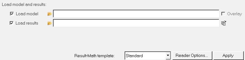
Figure 14. - Modeling window: The modeling window is the display area for your model. You can interact with the model in three-dimensional space in real time. In addition to viewing the model, entities can be selected interactively from the modeling window.
- Status bar: The status bar is located at the bottom of the screen. As you work in HyperView, any warning or error messages also display in the status bar, on the left side.
Define the Simulation Parameters and Import the Geometry
Start HyperMesh and Create a Model Database
In the next steps you will start HyperMesh and create the database for storage of the simulation settings.
-
Click OK.
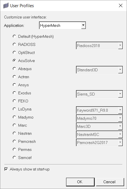
Figure 15.Traditional HyperMesh users will be able to tell the difference between the default HyperMesh profile and the CFD (AcuSolve) profile. There will be an additional CFD toolbar visible. Also, the Model Browser will be populated with some entities relevant to a CFD simulation setup.
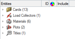
Figure 16.
Import the Geometry
-
Click .
Tip: Alternatively, click the arrow next to the Import Solver Deck icon
 on the standard
toolbar and select Import Geometry.
on the standard
toolbar and select Import Geometry. -
Select Parasolid as the File type.
Note: In general, if you are not sure about the geometry file type, leave the File type option as Auto Detect.
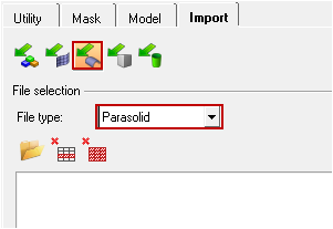
Figure 17. -
Click
 .
Note: If you see anything in the list of import files, clear the list before this step by clicking
.
Note: If you see anything in the list of import files, clear the list before this step by clicking .
. -
Click
 on the Visualization
toolbar to display the surfaces.
on the Visualization
toolbar to display the surfaces.
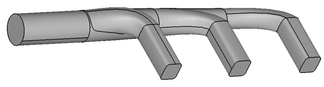
Figure 18.Tip: Use the following controls for visualizing the model:- Ctrl + Left-Click: Rotate the model
- Ctrl + Scroll: Zoom in/out
- Ctrl + Right Click: Pan the model
Define Mesh Controls and Generate the Mesh
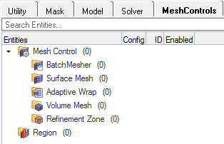
Figure 19.
The Mesh Controls Browser lets you access all of the different meshing technologies in the single browser. As you can see in the image above there are options to generate the surface mesh, volume mesh, refinement zones, and so on. Within these options there are associated model, local, feature, and refinement controls available. The model controls apply to the entire model. The local controls apply to a specific entity in the model, such as surfaces and elements.
You will start by creating a surface mesh control followed by a volume mesh control with active boundary layers. You will then add a volume mesh local control for the surfaces that do not require a boundary layer.
Set up the Surface Mesh Controls and Generate Surface Mesh
-
Under the Entity Selection group, click in the
field next to Entities then click the Surfaces
collector.

Figure 20.The surface entity selector menu opens in the menu area. -
Expand the Advanced group and verify the following
settings:
-
Mesh Connectivity: Keep
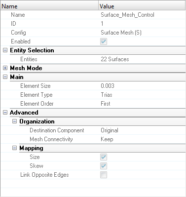
Figure 21.
-
Mesh Connectivity: Keep
Organize the Surfaces Elements
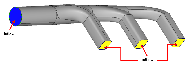
Figure 22.
-
In the dialog, click the Check none icon
 then activate the Inflow and
Outflow fields.
then activate the Inflow and
Outflow fields.
-
Click Create then Close.
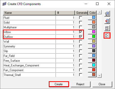
Figure 23. -
Open the Organize panel by doing one of the
following:
-
Click organize in the panel area.
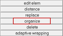
Figure 24. -
Click
 on the CFD
toolbar.
on the CFD
toolbar.
-
Click organize in the panel area.
-
In the modeling window, zoom in on the inlet surface
region and select any mesh element on the inlet surface.
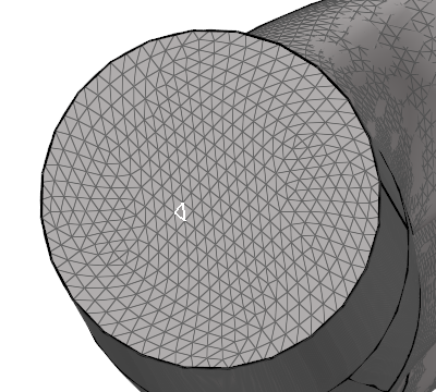
Figure 25. -
Similarly, select a mesh element on each of the Outflow surfaces then click on
the elems collector and select the by
face option. Verify that all the surface elements on the three
outlet surfaces are now highlighted then set the dest component
= to Outflow and click
move.
The model should now look similar to the figure below.
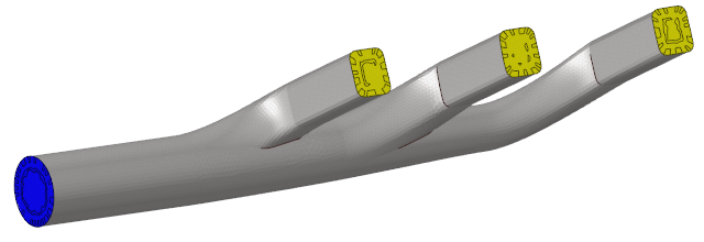
Figure 26.
Set up the Volume Mesh Controls
-
Under the Entity Selection group, click in
the value field next to Entities then click the
Components collector.

Figure 27.The Select Components dialog opens. -
Select all three components in the dialog and click
OK.
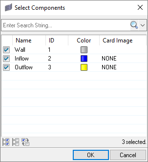
Figure 28.You can click the
 icon in the dialog to quickly select all of the
components.
icon in the dialog to quickly select all of the
components. -
Expand the Boundary Layer
group and set the boundary layer parameters as follows:
-
Change Hexa Transition Mode to All Prism
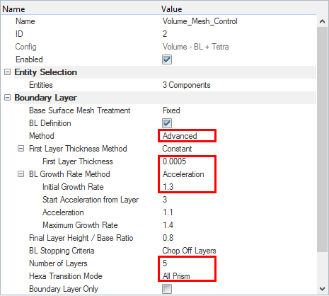
Figure 29.When generating boundary layer meshes in HyperMesh, it is recommended to use All Prism as the boundary layer meshing mode for superior element quality. The prism elements can later be split into tetrahedral elements, which is the recommended element type for AcuSolve.
This completes the boundary layer mesh control. You will now add a local control for surfaces that do not require a boundary layer.
-
Change Hexa Transition Mode to All Prism
-
Under the Entity Selection group, click in
the value field next to Entities then click the
Components collector.
Figure 30.The Select Components dialog opens. -
Select Inflow and Outflow from
the list and click OK.
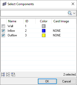
Figure 31. -
Expand the Boundary
Layer group and set Base Surface Mesh Treatment to
Float.
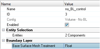
Figure 32. -
Finally, add a volume selector control to
put the boundary layer and the core tetra mesh in the same component.
-
In the Entity Editor,
activate the check box for BL and Tetras in One
Component.
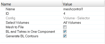
Figure 33.
-
In the Entity Editor,
activate the check box for BL and Tetras in One
Component.
Generate the Volume Mesh
In the previous steps, you created some model and local mesh controls. Your Mesh Controls Browser should look like the figure below.
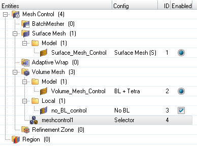
Figure 34.
When you set up the mesh controls, at least one active model control should be present before you generate the mesh. You can create multiple model controls, but only one model control can be active at a time. Surface and volume mesh however have different mesh controls.
Local controls are optional. You can create multiple local mesh controls, however only the ones which are selected at the time of mesh generation will be applied.
-
Right-click on Volume Mesh and click
Mesh.
The generated volume mesh is placed in a single collector called CFD_tetcore001 under the list of components. This collector will be visible in the Model Browser. Once the meshing is complete, observe the mesh using the visualization controls.
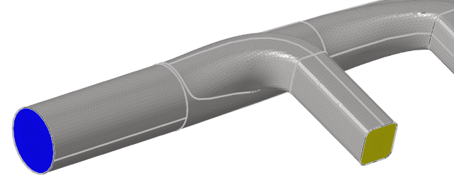
Figure 35.You can turn off the surface display to view the mesh more clearly. On the Visualization toolbar, click the
 icon
to display the geometry as wire frame. This will turn off the surface
display. To turn on the surface display, click the
icon
to display the geometry as wire frame. This will turn off the surface
display. To turn on the surface display, click the  icon. Zoom in to observe the boundary layer generated.
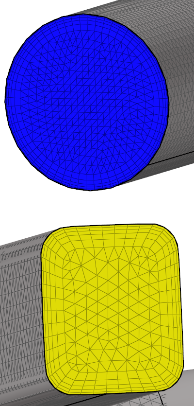
Figure 36. -
Click split.
Observe the mesh after the splitting process is complete.
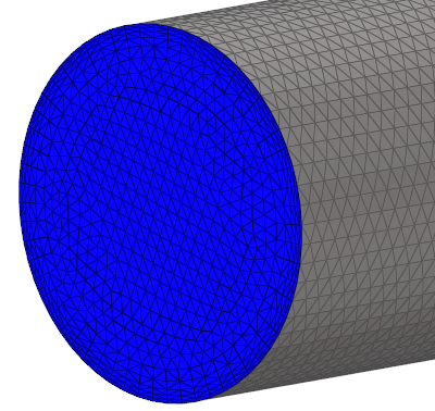
Figure 37.
Set up Simulation Parameters for AcuSolve
The next step after creating the mesh is to set up the simulation parameters. You will use the Solver Browser for this purpose. The Solver Browser provides a solver perspective view of the model structure in flat, listed tree structure.
Set General Simulation Parameters
-
Click to open the Solver Browser.
The Solver Browser lists every entity mapped to the active solver profile within the session and places those entities into their respective entity group folders.
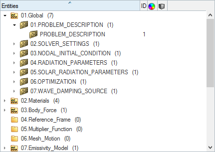
Figure 38. -
Change the Turbulence model from Laminar to Spalart
Allmaras.
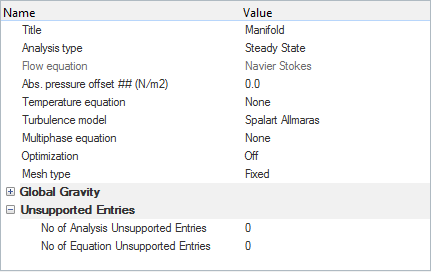
Figure 39.
Specify the Solver Settings
-
Check that Flow and Turbulence are set to On.
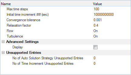
Figure 40.
Set Nodal Initial Conditions
-
Set the Eddy viscosity to 1e-05 m2/sec.
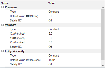
Figure 41.
Apply Volume Parameters
Volume groups are containers used for storing information about a volume region. This information includes solution and meshing parameters applied to the volume and the geometric regions that these settings are applied to.
There is one volume collector in this model, fluid. In the next steps you will set the material properties for it.
-
Select Water_HM and click
OK.
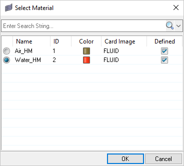
Figure 42.
Apply Surface Parameters
Surface groups are containers used for storing information about a surface, including solution and meshing parameters, and the corresponding surface in the geometry that the parameters will apply to.
-
In the Solver Browser, expand
12.Surfaces then expand the
WALL surface group. Click Wall
to open it in the Entity Editor. Verify that the Type is
set to WALL.
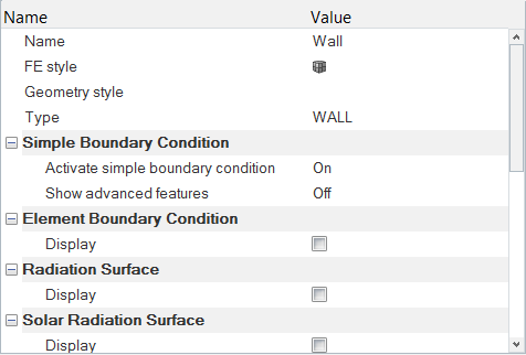
Figure 43. -
Expand the OUTFLOW surface group then click
Outflow to open it in the Entity Editor. Verify that the Type is set to
OUTFLOW.
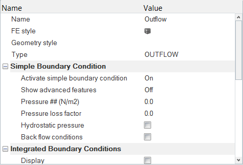
Figure 44. -
Expand the INFLOW surface group then click
Inflow to open it in the Entity Editor. Verify that the Type is set to
INFLOW. Set Inflow type to Average
velocity. Set the Average velocity to 2
m/sec.
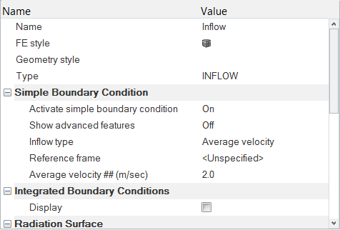
Figure 45.
Compute the Solution and Review the Results
Run AcuSolve
In this step, you will launch AcuSolve directly from HyperMesh and compute the solution.
-
In the Model Browser, ensure that the visibility of the
mesh for all collectors to be exported to AcuSolve
is activated. In this case, Fluid, Wall, Inflow and Outflow should be
activated.
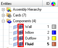
Figure 46.The display of the mesh icon beside the component name indicates that the visibility of mesh for that component is on. The display of the mesh of a component can be turned on/off by clicking on that icon.
-
Click
 on the ACU toolbar.
The Solver job Launcher dialog opens.
on the ACU toolbar.
The Solver job Launcher dialog opens.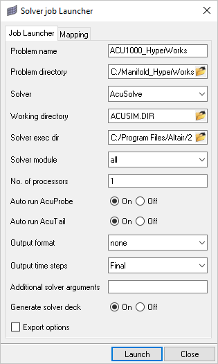
Figure 47.For this case, the default settings will be used. You may choose to change the number of processors to allow AcuSolve to run using more processors (4 or 8), if available. HyperMesh will generate the required solver input files and launch AcuSolve. AcuSolve will calculate the steady state solution for this problem.
-
Click Launch to start the
solution process.
As the solution progresses, an AcuTail and an AcuProbe dialog will open. Solution progress is reported in the AcuTail dialog. An AcuSolve Control dialog will also open from which you can control the solution process. In this dialog you have options to stop the solution or generate the output files at the end of the current time step.
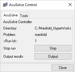
Figure 48.A summary of the run printed in the AcuTail dialog indicates that AcuSolve has finished running the solution.
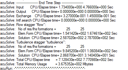
Figure 49.
Monitor the Solution with AcuProbe
-
Right-click on Final and select Plot
All.
Note: You might need to click
 on the toolbar in order to
properly display the plot.
on the toolbar in order to
properly display the plot.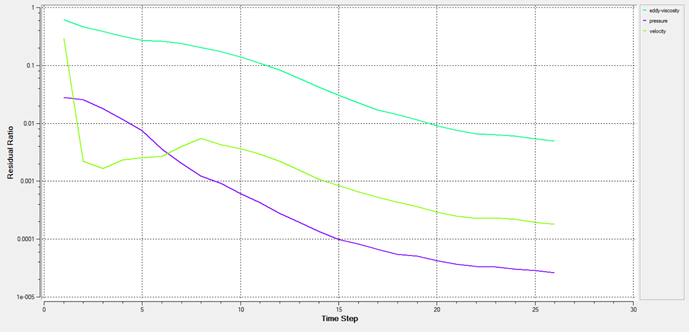
Figure 50.The plot above shows the residuals of the equations as the solution progresses through each time step. You can see the residuals dropping smoothly. Once the pressure and velocity residual ratios reach a value less than the specified convergence tolerance (0.001), the solution is considered to be converged. By default, the eddy viscosity convergence tolerance is set to a magnitude of one order higher than the specified convergence tolerance (0.01).
Post-Process the Results with HyperView
Open HyperView and Load the Model and Results
-
In the Load model and results panel, click
 next
to Load model.
next
to Load model.
Apply Pressure Contours on the Boundary Surfaces
-
Click
 on the Results toolbar to open the Contour panel.
-
Click Apply.
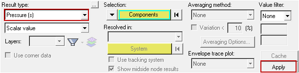
Figure 51. -
In the panel area, under the Display tab, turn off
the Discrete color option.
Figure 52. -
Click the Legend tab then
click Edit Legend. In the dialog, change the Numeric
format to Fixed then click
OK.
The pressure contour should be displayed as shown in the figure below.
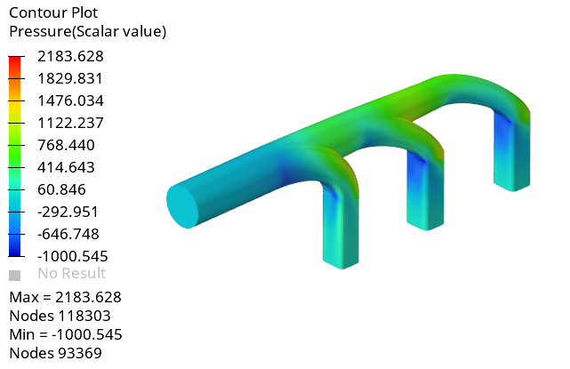
Figure 53.
Save Plots as Image Files
-
On the Image Capture toolbar toggle the
 /
/ icons so that it shows the icon to save to file.
-
Click the
 icon on the Image Capture
toolbar.
icon on the Image Capture
toolbar.
-
Provide a name for the image in the dialog and click
Save.
If you want to use the image in a presentation you can copy them to the clipboard by toggling the Save Image to File/Clipboard icon to instead of . Then paste the image in your
presentation.
Create Pressure and Velocity Contours on a Cut Plane
-
For the Base coordinates, enter a value of -0.015 for
the Y-coordinate and press Enter.
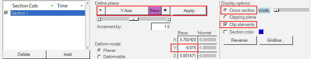
Figure 54. -
In the dialog, uncheck the Show option under Gridline
then click OK.
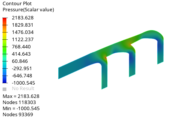
Figure 55. -
Click
on the Results toolbar to open the Contour panel.
-
Click Apply.
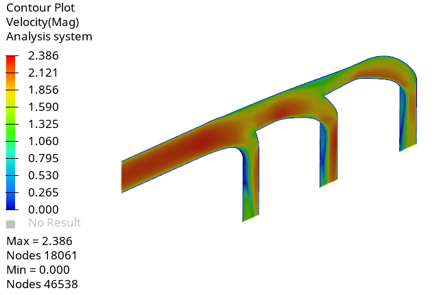
Figure 56.
Create a Clipping Plane
-
In the Section Cut panel change the selection under Display
options from Cross section to Clipping plane.
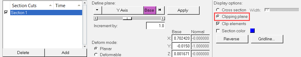
Figure 57. -
Click Reverse to toggle the clipping direction to your
choosing.
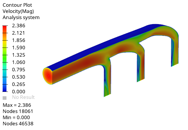
Figure 58.
Create Velocity Vectors
-
Click the
 icon on the Results
toolbar.
icon on the Results
toolbar.
-
Click Displayed.
Figure 59. -
Select the Z+X Resultant option.
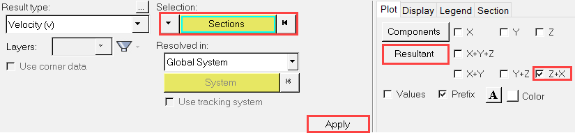
Figure 60. -
Click the Display tab and set the options as shown in
the figure below.
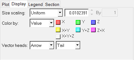
Figure 61. -
Set the Number of rows and columns to 20 and
50 respectively then click
Apply.
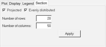
Figure 62.The vector plot should be displayed as shown in the figure below.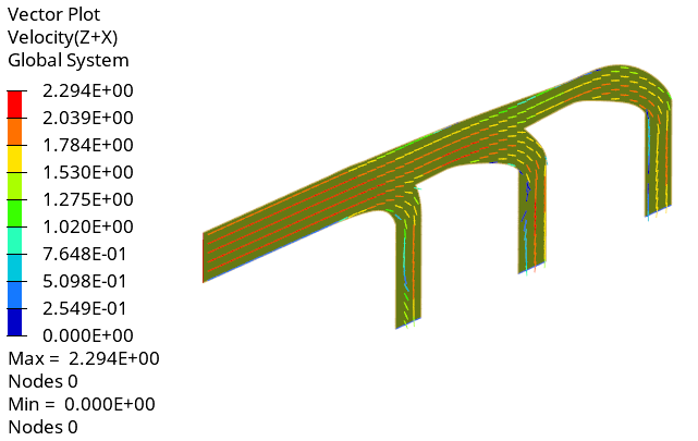
Figure 63.
Display Streamlines
-
Click the
 icon next to Section 1 to turn
off its display.
icon next to Section 1 to turn
off its display.
-
Click the
 icon on the Results toolbar to
open the Streamlines panel.
icon on the Results toolbar to
open the Streamlines panel.
-
Click the
 icon.
The Reference point dialog opens.
icon.
The Reference point dialog opens. -
Enter the reference points as shown in the figure below.
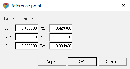
Figure 64. -
Enter the Streamline Size as 3 and press Enter .
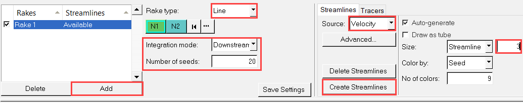
Figure 65.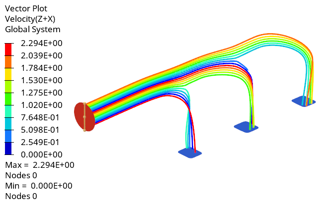
Figure 66.
Summary
In this tutorial, you worked through a basic workflow to carry out a CFD simulation and post-processed the results using HyperWorks products, namely HyperMesh and HyperView. You started by importing and meshing the model in HyperMesh. You also set up the model and launchedAcuSolve directly from within HyperMesh. Upon completion of the solution by AcuSolve, you used HyperView to post-process the results. You learned how to create contours on the boundary surfaces and the section cuts, velocity vectors, and streamlines.