ACU-T: 2300 Atmospheric Boundary Layer Problem – Flow Over Building
Prerequisites
Prior to starting this tutorial, you should have already run through the introductory HyperWorks tutorial, ACU-T: 1000 HyperWorks UI Introduction. To run this simulation, you will need access to a licensed version of HyperMesh and AcuSolve.
Prior to running through this tutorial, click here to download the tutorial models. Extract ACU-T2300_Building.hm from HyperMesh_tutorial_inputs.zip.
Since the HyperMesh database (.hm file) contains meshed geometry, this tutorial does not include steps related to geometry import and mesh generation.
Problem Description
The problem to be addressed in this tutorial is shown schematically in Figure 1. As an example, this problem shows the capability of Atmospheric Boundary Layer modelling in AcuSolve.
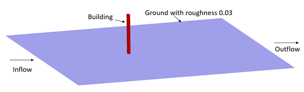
Figure 1.
In this tutorial, you will simulate the air flow over a building with a ground roughness of 0.03. In this case, User Defined Atmospheric Roughness Type is considered.
Open the HyperMesh Model Database
-
Click the Open Model icon
 located on the standard toolbar.
The Open Model dialog opens.
located on the standard toolbar.
The Open Model dialog opens.
Set the General Simulation Parameters
-
Set the Turbulence Model to Spalart Allmaras.
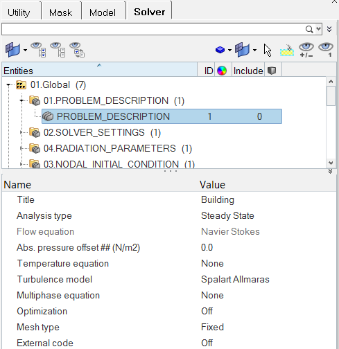
Figure 2. -
Set the Relaxation Factor to 0.4.
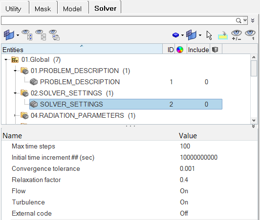
Figure 3.
Set Up Boundary Conditions and Material Model Parameters
In this step, you will define the Boundary Conditions (BCs) for the problem and assign material properties to the fluid volume.
Set Up Material Model Parameters
-
Set the Material Type to FLUID if it's not already set.
Leave the remaining default values as is.
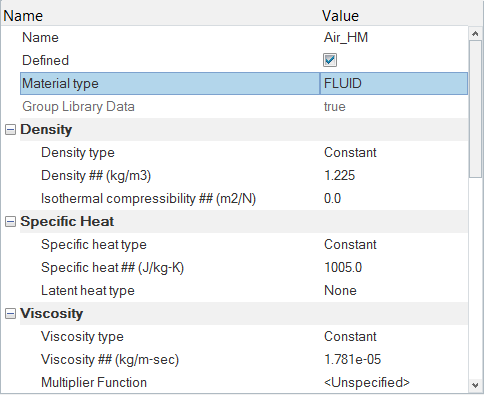
Figure 4.
Set Up Fluid Volume Material
-
Set the Material to Air_HM.
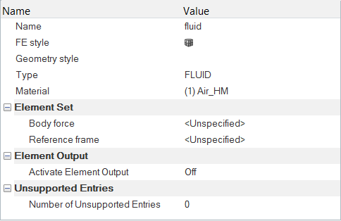
Figure 5.
Set Up Boundary Conditions
-
In the Solver Browser, expand then click on Inflow. In the Entity Editor,
- Set the Type to INFLOW.
- Set the Inflow Type to Atmospheric.
- Set the Atmospheric Roughness Type to User value.
- Set the Atmospheric Ground Roughness to 0.001.
- Set the Atmospheric Reference Vel Type to Friction velocity.
- Set the Atmospheric Friction Velocity to 0.106.
- For Atmospheric Ground Origin, set the coordinates to (0, 0, 0).
- For Atmospheric Ground Normal Direction, set the coordinates to (0, 0, 1).
- For Atmospheric Flow Direction, set the coordinates to (1, 0, 0).
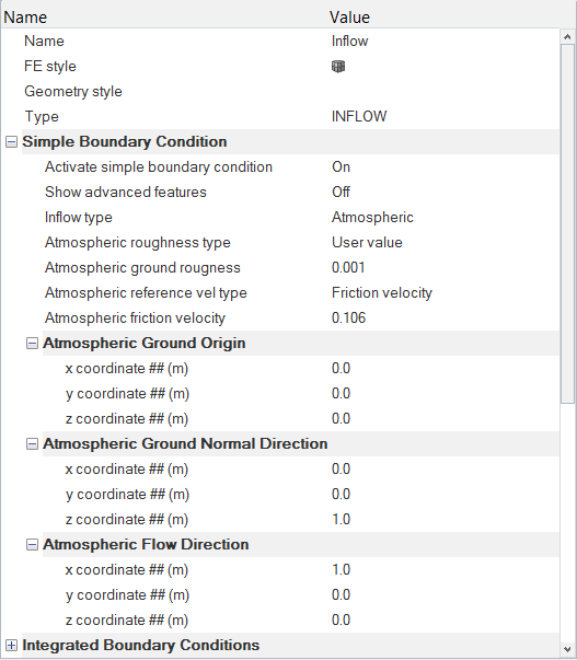
Figure 6. -
Expand OUTFLOW then click on
Outflow. In the Entity Editor, change the Type to OUTFLOW.
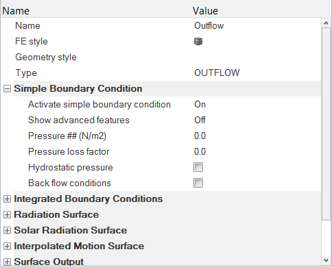
Figure 7. -
Expand WALL then click on
Building. In the Entity Editor, change the Type to WALL.
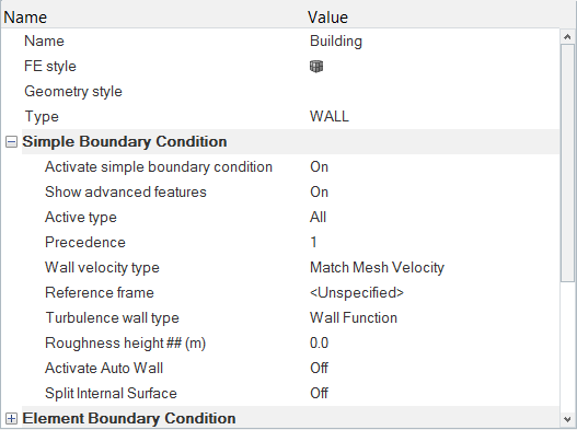
Figure 8. -
Under WALL, click on Wall. In the
Entity Editor,
- Change the Type to WALL.
- Set the Roughness height to 0.03.
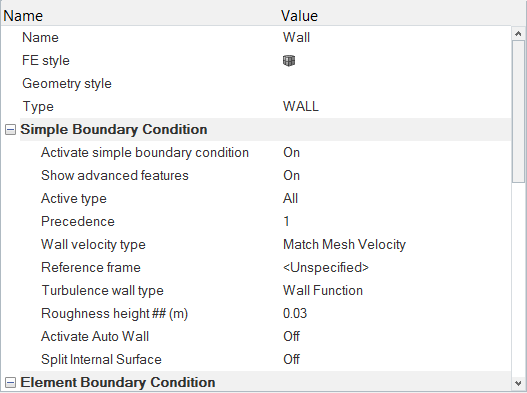
Figure 9. -
Expand SLIP then click on Slip.
In the Entity Editor, change the Type to
SLIP.
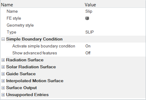
Figure 10.
Set Up Nodal Initial Conditions
-
Change the Eddy viscosity to 0.0001
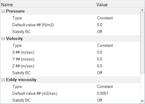
Figure 11.
Compute the Solution
In this step, you will launch AcuSolve directly from HyperMesh and compute the solution.
Run AcuSolve
-
Click
 on the ACU toolbar.
The Solver job Launcher dialog opens.
on the ACU toolbar.
The Solver job Launcher dialog opens. -
Leave the remaining options as
default and click Launch to start the solution
process.
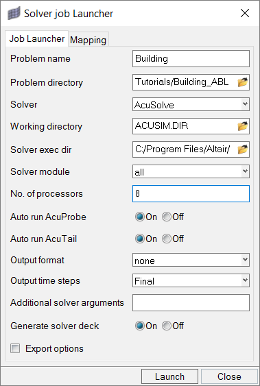
Figure 12.
Post-Process the Results with HyperWorks HV
Start HyperView from the Windows Start menu by clicking .
Load Model and Results
- Once the HyperWorks HV window is loaded, click .
-
In the Load model and results panel, click
 next
to Load model.
next
to Load model.
- In the Load Model File dialog, navigate to your working directory and select the AcuSolve .Log file for the solution run that you want to post-process. In this example, the file to be selected is Building.1.Log.
- Click Open.
- Click Apply in the panel area to load the model and results.
Coordinate the Surface for Showing Velocity Magnitude on the Y Plane
-
From the View Controls toolbar, click
 to create a new coordinate surface on the y
plane.
to create a new coordinate surface on the y
plane.
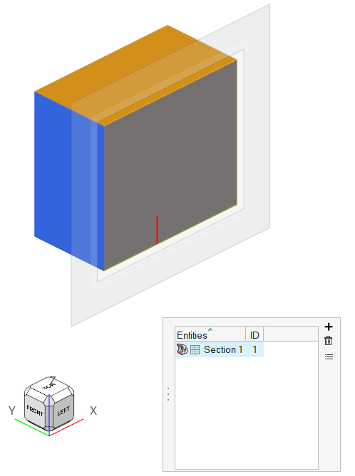
Figure 13. -
Click
 in the microdialog to only display the section cut.

Figure 14. -
Click the Left face on the View Cube to orient the
section cut.
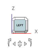
Figure 15. -
From the Results ribbon, click the Contour tool.

Figure 16. -
Click Apply.
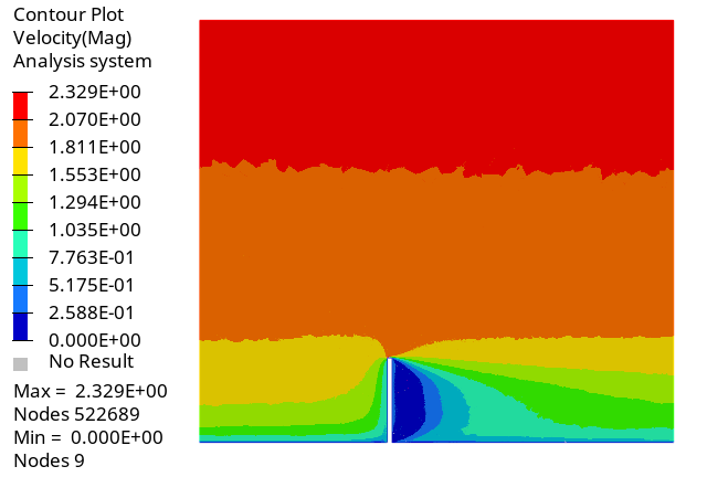
Figure 17.
Coordinate the Surface for Showing Velocity Vectors on the Y Plane
-
From the Results ribbon, click the Vector tool.

Figure 18. -
Click the arrow next to the Components entity selector
and select Sections.
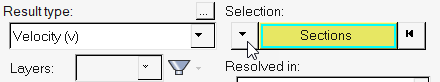
Figure 19. -
Activate X+Y+Z for Resultant.
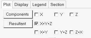
Figure 20. -
Set Size scaling to 0.05.
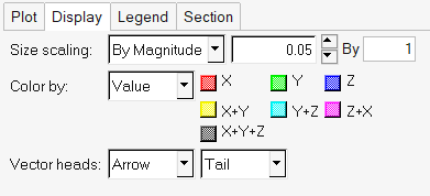
Figure 21. -
Click Apply.
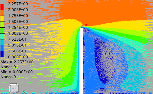
Figure 22.
Summary
In this tutorial, you worked through a basic workflow to set up a CFD model, carry out a CFD simulation, then post-process the results using HyperWorks products, namely AcuSolve, HyperMesh and HyperWorks HV. You started by importing the model in HyperMesh. Then, you defined the simulation parameters and launched AcuSolve directly from within HyperMesh. Upon completion of solution by AcuSolve, you used HyperWorks HV to post-process the results and create contour and vector plots.