ACU-T: 3202 Heat Transfer Between Concentric Spheres – P1 Radiation Model
Prerequisites
This tutorial provides the instructions for setting up, solving, and viewing results for a steady state simulation of radiation heat transfer between concentric spheres using the P-1 Radiation model. Prior to starting this tutorial, you should have already run through the introductory HyperWorks tutorial, ACU-T: 1000 HyperWorks UI Introduction, and have a basic understanding of HyperWorks CFD and AcuSolve. To run this simulation, you will need access to a licensed version of HyperWorks CFD and AcuSolve.
Prior to running through this tutorial, click here to download the tutorial models. Extract ACU-T3202_P1Rad.hm from HyperWorksCFD_tutorial_inputs.zip.
Problem Description
The problem to be addressed in this tutorial is shown schematically in Figure 1. In this problem, a P1 radiation model is used to simulate the heat transfer due to radiation between concentric spheres. The inside surface of the inner and the outside surface of the outer sphere are both held at constant temperature while the gap between them radiates the heat from one sphere to the other.
The problem consists of a fluid region with arbitrary material properties between two concentric spheres with surfaces held at fixed temperature, as shown in the following figure, which is not drawn to scale. The radius of the outer sphere is 0.04 m and the radius of the inner sphere is 0.01 m. The inner surface of the inner sphere is defined to have a constant wall temperature at 300.0 K (26.85 ºC). The outer surface of the outer sphere is defined to have a constant wall temperature at 1300.0 K (1026.85 ºC). The fluid within the spheres is defined as a non-conducting material, allowing heat to transfer via radiation only.
The problem is solved as a steady state case to allow the heat transfer in the solid and fluid regions to reach an equilibrium.
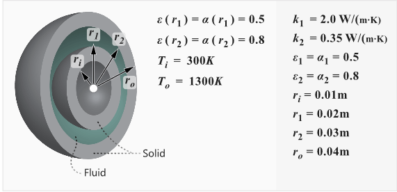
Figure 1.
Start HyperWorks CFD and Open the HyperMesh Database
-
From the Home tools, Files tool group, click the Open Model tool.

Figure 2.The Open File dialog opens.
Validate the Geometry
The Validate tool scans through the entire model, performs checks on the surfaces and solids, and flags any defects in the geometry, such as free edges, closed shells, intersections, duplicates, and slivers.
Figure 3.
Set Up Flow
Set Up the Simulation Parameters and Solver Settings
-
From the Flow ribbon, click the Physics tool.

Figure 4.The Setup dialog opens. -
Under the Physics models setting:
- Set Time marching to Steady.
- Set the Turbulence model to Laminar.
- Activate the Heat transfer checkbox.
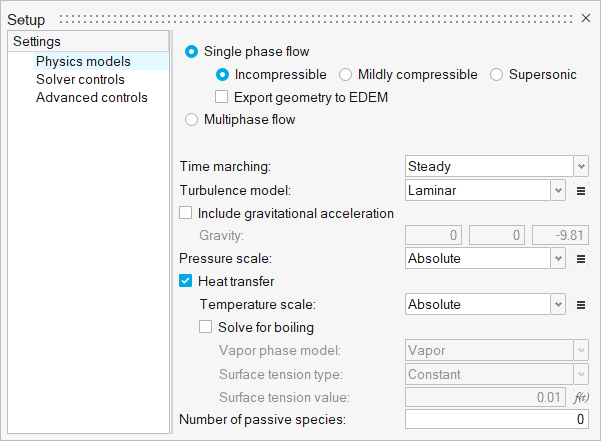
Figure 5. -
Deactivate the Flow checkbox.
In this tutorial, you will only be solving for the temperature field.
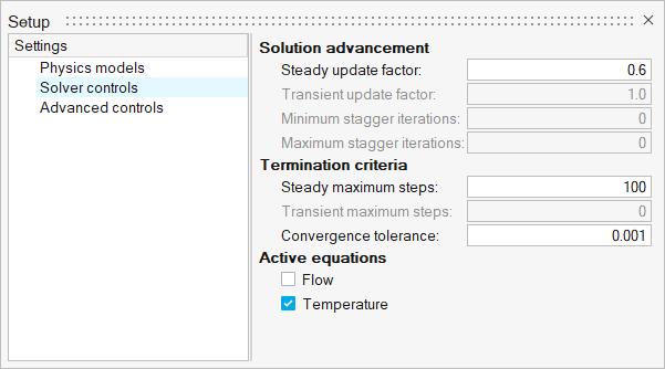
Figure 6.
Create Material Models
-
From the Flow ribbon, click the Material Library tool.

Figure 7.The Material Library dialog opens. -
Click
 to create a new material.
-
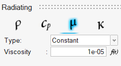
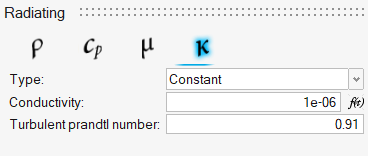
Enter the following values for each of the material property tabs then close
the dialog.
- Density – 1000 kg/m3
- Specific Heat – 10000 J/kg-K
- Viscosity – 1e-5 kg/m-sec
- Conductivity – 1e-6 W/m-K
Figure 8.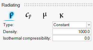

Assign Material Properties
-
From the Flow ribbon, click the Material tool.

Figure 9. -
Select the outer solid and assign the Outer material
model from the microdialog.
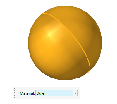
Figure 10. -
On the guide bar, click
 to execute the command and remain in the
tool.
to execute the command and remain in the
tool.
-
On the guide bar, click
 .
.
-
On the guide bar, click
 to execute
the command and exit the tool.
to execute
the command and exit the tool.
Assign the Flow Boundary Conditions
-
From the Flow ribbon, click the No Slip tool.

Figure 11. -
Select the two faces remaining in the modeling window.
In the microdialog, assign a
Temperature boundary condition at
300 K.
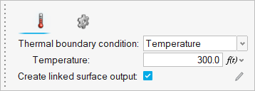
Figure 12. -
On the guide bar, click
to execute the command and remain in the
tool.
-
On the guide bar, click
to execute
the command and exit the tool.
Set Up Radiation
Select the Radiation Model
-
From the Radiation ribbon, Thermal Radiation tools, click the Physics tool.

Figure 13.The Radiation Settings dialog opens. -
Activate the Thermal radiation checkbox and set the
Radiation model to P1 Model.
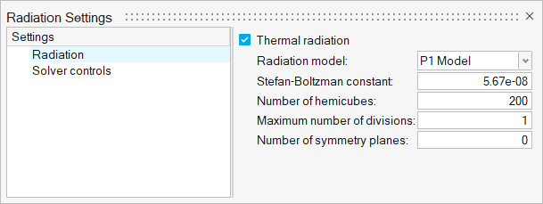
Figure 14.
Define the Radiation Material Properties
-
Click the Surface Finish Library tool.
Figure 15.The Surface finish library opens. -
Click .
-
Similarly, create another Emissivity model named Outer
with an Emissivity of 0.8.
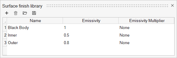
Figure 16. -
From the Participating Media tools, click the
Model tool.
Figure 17.The Participating media model library opens. -
Click and create a model with the following properties.
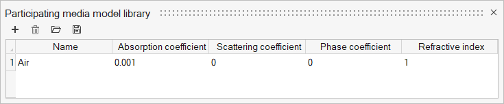
Figure 18.
Assign the Participating Media Model
-
From the Participating Media tools, click the
Assign tool.

Figure 19. -
Click on the guide bar.
Assign the Emissivity Model
-
From the Thermal Radiation tools, click the
Surface Finish
tool.

Figure 20. -
Click on the guide bar.
-
Click
 on the guide bar.
Generate the Mesh
-
From the Mesh ribbon, click the
Volume tool.

Figure 21.The Meshing Operations dialog opens.Note: If the model has not been validated, you are prompted to create the simulation model before running the batch mesh. -
Accept all other default parameters.
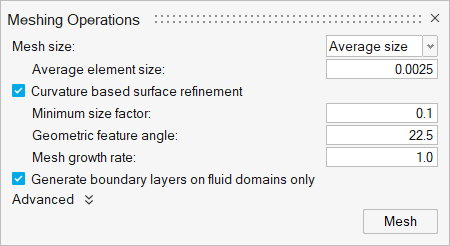
Figure 22.
Run AcuSolve
-
From the Solution ribbon, click the Run tool.

Figure 23. -
Leave the remaining options as default and click
Run to launch AcuSolve.
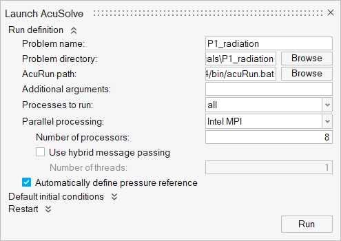
Figure 24. -
In the Plot Utility dialog, double-click on
Residual Ratio to plot the residuals.
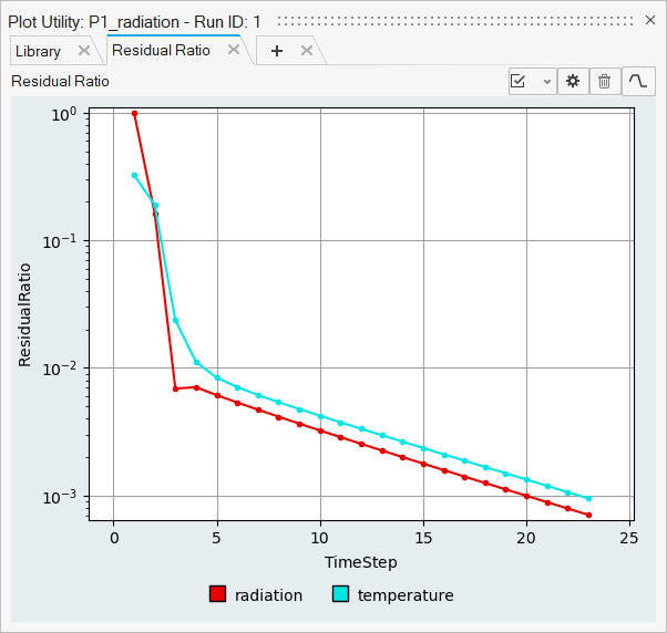
Figure 25.
Post-Process the Results with HW-CFD Post
-
In the browser, click the icon beside Flow Boundaries to turn off the display
of all the surfaces.
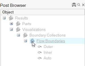
Figure 26. -
Click the Slice Planes tool.

Figure 27. -
In the slice plane microdialog, click
 to
create the slice plane.
to
create the slice plane.
-
Click
 and set the Colormap Name to Rainbow
Uniform.
and set the Colormap Name to Rainbow
Uniform.
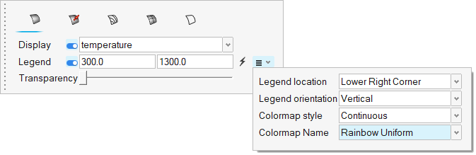
Figure 28. -
Click on the guide bar then press F
to fit the section cut to the screen.
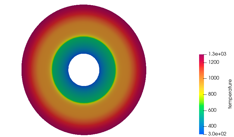
Figure 29.
Summary
In this tutorial, you learned how to set up and solve a radiation heat transfer simulation using the P1 radiation model. You started by importing the HyperWorks CFD input database and defining the flow and radiation setup. Then, you generated the mesh and submitted the AcuSolve simulation. Once the solution was computed, you created a plot of residual ratios using the plot utility in HyperWorks CFD. Finally, you created a contour plot of temperature distribution on a section cut using HyperWorks CFD Post.