ACU-T: 4000 Transient Dam Break Simulation
Prerequisites
This tutorial provides instructions for setting, solving and viewing results for a transient dam break simulation using the Level Set method. Prior to starting this tutorial, you should have already run through the introductory HyperWorks tutorial, ACU-T: 1000 HyperWorks UI Introduction, and have a basic understanding of HyperMesh, AcuSolve, and HyperView. To run this simulation, you will need access to a licensed version of HyperMesh and AcuSolve.
Prior to running through this tutorial, click here to download the tutorial models. Extract ACU-T4000_DamBreak.hm from HyperMesh_tutorial_inputs.zip.
Since the HyperMesh database (.hm file) contains meshed geometry, this tutorial does not include steps related to geometry import and mesh generation.
Problem Description
The problem to be addressed in this tutorial is shown schematically in the figure below. It consists of a square water column held in place by the reservoir walls. At time t=0, the walls are removed and the water column is now free to flow out. The simulation can be used to visualize and study the surge patterns as the column of water rushes out, as in a dam wall break.

Figure 1.
Open the HyperMesh Model Database
-
Click the Open Model icon
 located on the standard toolbar.
The Open Model dialog opens.
located on the standard toolbar.
The Open Model dialog opens.
Set the Transient Simulation Parameters
Set the Analysis Parameters
-
Set the Multiphase equation to Level Set.
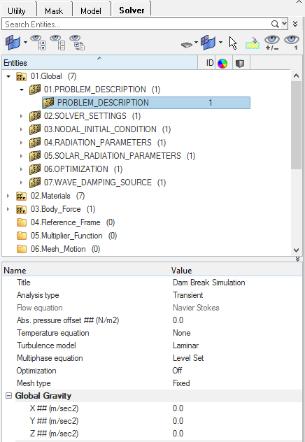
Figure 2.
Specify the Solver Settings
-
Check that the Flow and Field options are turned On.
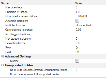
Figure 3.
Define the Nodal Outputs
-
In the Entity Editor, set the Time step frequency to
1 and toggle on the Output initial condition
field.
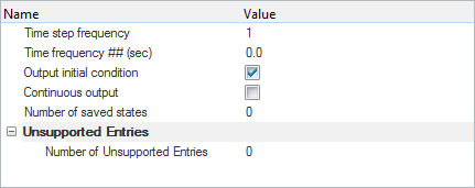
Figure 4.
Create a Multiphase Model and Set the Body Force
Create a Multiphase Material Model
-
Enter Water as the Field 2 name.
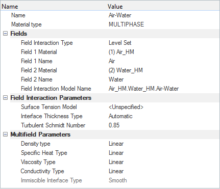
Figure 5.
Set the Body Force
-
In the Entity Editor, set the Y gravity to
-9.81 m/sec2 and Z gravity to
0.0.
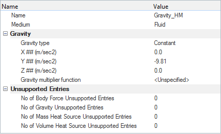
Figure 6.
Set the Nodal Initial Conditions and Boundary Conditions
In this step, you will start by creating a node-set for assigning nodal initial conditions for volume fraction. All the nodes in the set are assigned a volume fraction of 1 for water, thereby creating a water column.
Create a Node Set
- Go to the Model Browser, right-click on empty space in the browser area, and select .
- In the Entity Editor, rename the set to Water_Column.
Set the Boundary Conditions
-
Click z_pos. In the Entity Editor, change the Type to SYMMETRY.
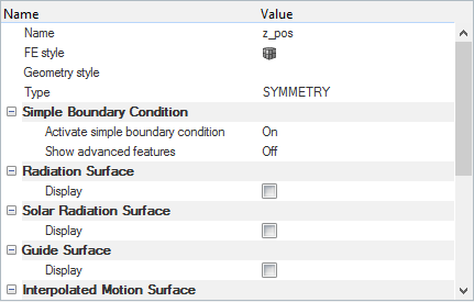
Figure 7. -
Click sides. In the Entity Editor, verify that the Type is set to WALL.
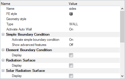
Figure 8. -
Click Fluid. In the Entity Editor,
- Change the Type to MULTIPHASE.
- Select Air-Water as the Material.
- Select Gravity_HM as the Body Force.
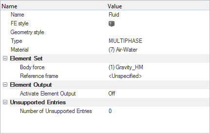
Figure 9.
Assign Reference Pressure
-
Click on the Node collector. Then, in the graphics
window, click on a node in the Fluid volume.
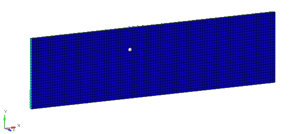
Figure 10. -
Change the Boundary condition variable to Pressure and
leave the remaining settings as default.
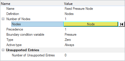
Figure 11.
Set the Nodal Initial Conditions
-
Set the Initial Volume Fraction to 1.0.
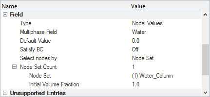
Figure 12.
Assign Nodes to the Node Set
-
Toggle on the Water_Column block then click
select.
All the nodes in the Water column block are highlighted in the graphics area.
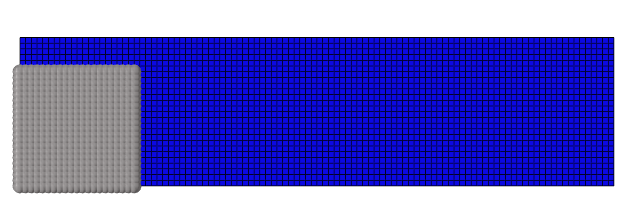
Figure 13.
Compute the Solution
In this step, you will launch AcuSolve directly from HyperMesh and compute the solution.
Run AcuSolve
-
Click
 on the ACU toolbar.
The Solver job Launcher dialog opens.
on the ACU toolbar.
The Solver job Launcher dialog opens. -
Leave the remaining options as
default and click Launch to start the solution
process.
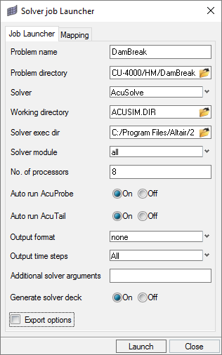
Figure 14.
Post-Process the Results with HyperView
Open HyperView and Load the Model and Results
-
In the Load model and results panel, click
 next
to Load model.
next
to Load model.
Create the Water Flow Animation
In this step, you will create an animation of the water flow as it surges once the walls restricting the water column are removed.
-
Orient the display to the xy-plane by clicking
 on the Standard Views toolbar.
-
Click
 on the Results toolbar to open the Contour panel.
-
In the Edit Legend dialog, change the Number of levels to
2 and the Numeric format to
Fixed.
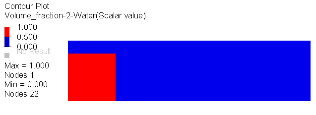
Figure 15. -
On the Animation toolbar, click the Animation Controls icon
 .
.
-
Click the Start/Pause Animation icon
 to play the animation in the graphics area.
Save the Animation
-
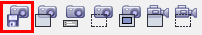
On the ImageCapture toolbar, make sure that the Save Image to File option is
On.
-
Click the Capture Graphics Area Video icon
 .
The Save Graphics Area Video As dialog opens.
.
The Save Graphics Area Video As dialog opens.
Summary
In this tutorial, you successfully learned how to set up and solve a multiphase flow problem using HyperMesh and AcuSolve. You also learned how to create a multiphase model using the Level Set method. Once the solution was computed, you post-processed the results in HyperView where you generated an animation of the water flow as it surged once the dam walls were removed.