ACU-T: 4200 Humidity – Pipe Junction
Prerequisites
Prior to starting this tutorial, you should have already run through the introductory HyperWorks tutorial, ACU-T: 1000 HyperWorks UI Introduction. To run this simulation, you will need access to a licensed version of HyperMesh and AcuSolve.
Prior to running through this tutorial, click here to download the tutorial models. Extract ACU-T4200_Humidity.hm from HyperMesh_tutorial_inputs.zip.
Since the HyperMesh database (.hm file) contains meshed geometry, this tutorial does not include steps related to geometry import and mesh generation.
Problem Description
The problem to be addressed in this tutorial is shown schematically in Figure 1. As an example, a pipe junction problem is attached here to show the capability of the Humidity modelling in AcuSolve. In this problem, there are two inlets with different flow, thermal, and humidity conditions. As the flow proceeds downstream of the pipe, two pipes merge into a single pipe to create a single outlet and a distinct profile of temperature and humidity is attained. The geometry is symmetric about the XZ midplane of the pipe, as shown in the figure.
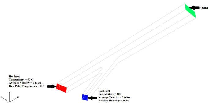
Figure 1.
Open the HyperMesh Model Database
-
Click the Open Model icon
 located on the standard toolbar.
The Open Model dialog opens.
located on the standard toolbar.
The Open Model dialog opens.
Set the General Simulation Parameters
Set the Analysis Parameters
-
Switch Humid Air Model to On.
This will automatically change the Multiphase equation to Advective Diffusive.
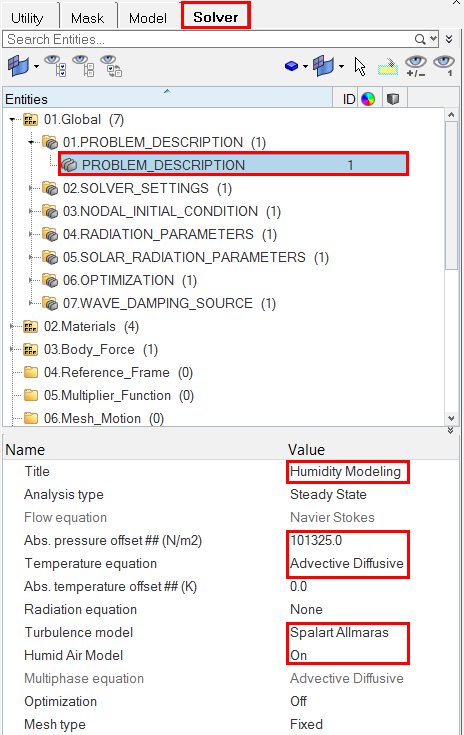
Figure 2. -
Set the Relaxation factor to 0.
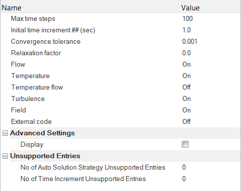
Figure 3.
Set Up Body Force Parameters
-
Set Gravity in the Y direction to -9.81
m/sec2 and change the Z direction to
0.
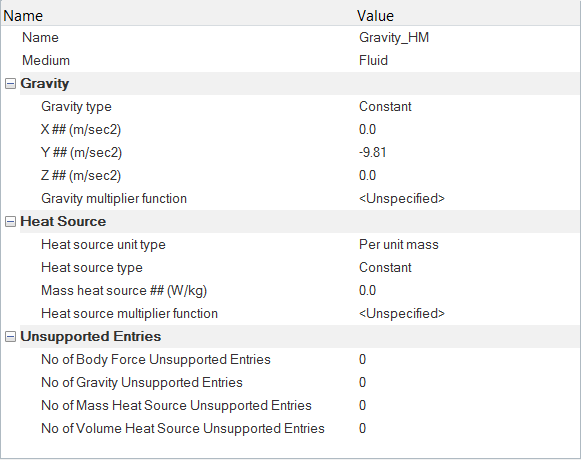
Figure 4.
Set Up Boundary Conditions and Nodal Initial Conditions
Set the Boundary Conditions
-
Click Hot_Inlet. In the Entity Editor,
- Change the Type to INFLOW.
- Set the Inflow type to Average velocity.
- Set the Average velocity to 1 m/s.
- Set the Temperature to 333.15 K.
- Set Incoming Humidity type to Dew Point Temperature and set the value to 278.15 K.
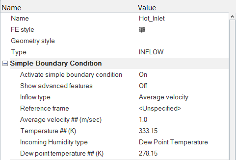
Figure 5. -
Click Cold_Inlet. In the Entity Editor,
- Change the Type to INFLOW.
- Set the Inflow type to Average velocity.
- Set the Average velocity to 3 m/s.
- Set the Temperature to 283.15 K.
- Set Incoming Humidity type to Relative Humidity and set the value to 20.
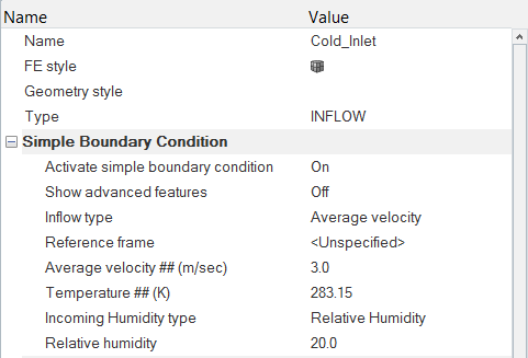
Figure 6. -
Click Outlet. In the Entity Editor, change the type to OUTFLOW.
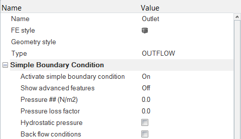
Figure 7. -
Click plusY. In the Entity Editor, change the type to SLIP.
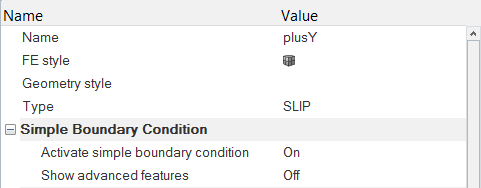
Figure 8. -
Click Walls. In the Entity Editor, verify that the Type is set to WALL.
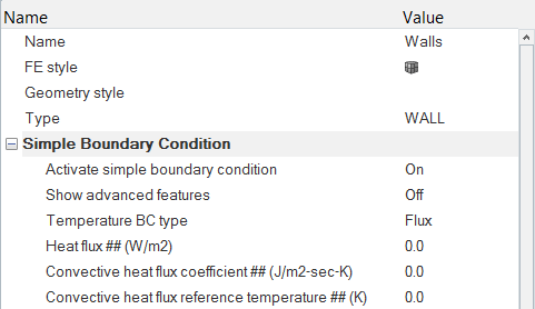
Figure 9. -
Click Fluid. In the Entity Editor,
- Change the Type to MULTIPHASE.
- Select HumidAir_HM as the Material.
- Set Body force to Gravity_HM.
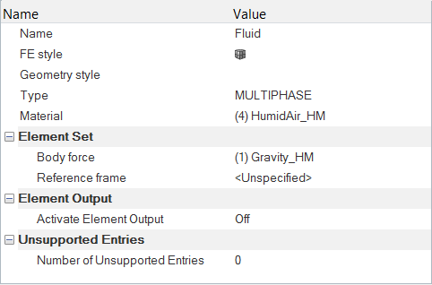
Figure 10.
Set the Nodal Initial Conditions
-
Change the Default value of Relative Humidity to
20.
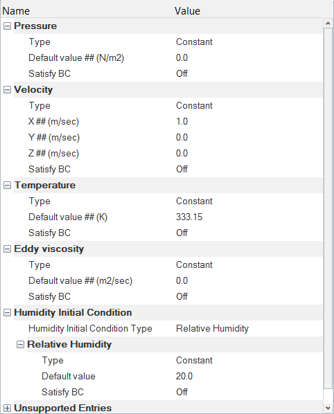
Figure 11.
Compute the Solution
In this step, you will launch AcuSolve directly from HyperMesh and compute the solution.
Run AcuSolve
-
Click
 on the ACU toolbar.
The Solver job Launcher dialog opens.
on the ACU toolbar.
The Solver job Launcher dialog opens. -
Leave the remaining options as
default and click Launch to start the solution
process.
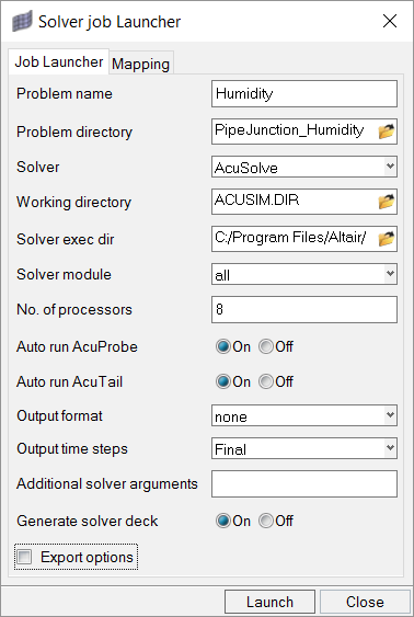
Figure 12.
Post-Process the Results with HyperView
Open HyperView and Load the Model and Results
-
In the Load model and results panel, click
 next
to Load model.
next
to Load model.
Create Contour Plots
-
Click the Isolate shown icon
 and then click on the minusY
component to turn off the display of all components except the minusY
component.
and then click on the minusY
component to turn off the display of all components except the minusY
component.
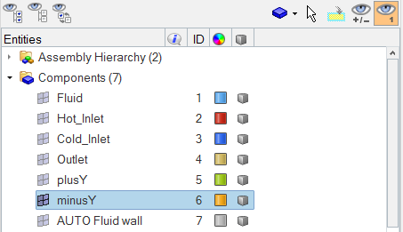
Figure 13. -
Orient the display to the xz-plane by clicking
 on the Standard Views toolbar.
-
Click
 on the Results toolbar to open the Contour panel.
-
In the panel area, under the Display tab, turn off
the Discrete color option.
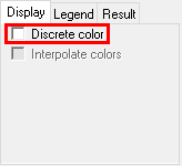
Figure 14. -
Verify that the contour looks like the figure below.
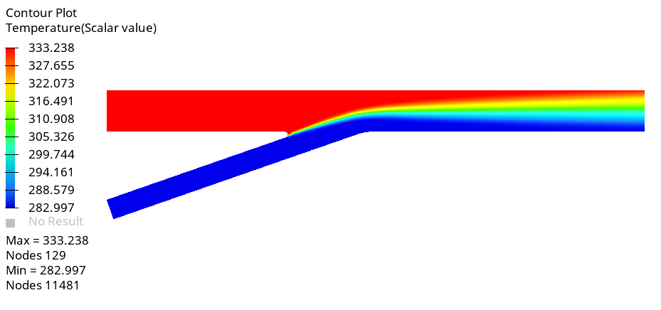
Figure 15. -
Change the Result type to Relative_humidity (v) then
click Apply to view the relative humidity contour on the
minus-Y plane.
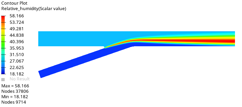
Figure 16. -
Change the Result type to
Mass_fraction-1-Humidity_HM.HumidAir(s) then click
Apply.
Use the range 0.001306 to 0.0406.
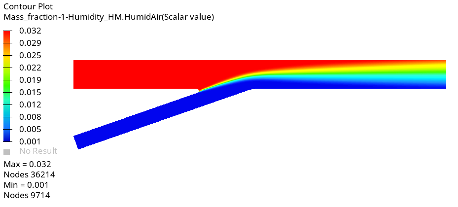
Figure 17. -
Change the Result type to Velocity (v) then click
Apply.
Use the range 0 to 3.753.
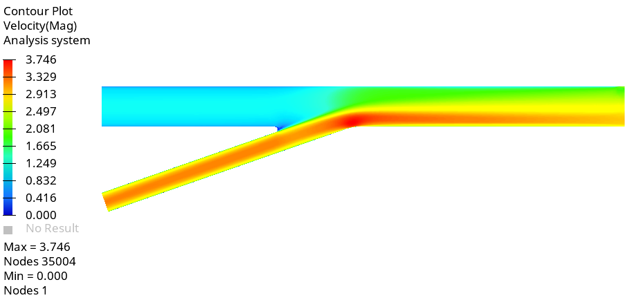
Figure 18.
Summary
In this tutorial, you worked through a basic workflow to set-up a CFD model, carried out a CFD simulation, and then post-processed the results using HyperWorks products, namely AcuSolve, HyperMesh and HyperView. You started by importing the model in HyperMesh. Then, you defined the simulation parameters and launched AcuSolve directly from within HyperMesh. Upon completion of the solution by AcuSolve, you used HyperView to post-process the results and create contour plots.