First Order Filter

A first order filter, with cutoff frequency R, is used to identify the dynamic component, x , of the input signal, X. The transfer functions of the signal sent to the dynamic and the static models, assuming X0=0, are:

TF of signal to dynamic model =

x(jω)X(jω)=ω2R2+ω2+jRωR2+ω2,j=1,ω=2πf=angularfrequency MathType@MTEF@5@5@+=feaagKart1ev2aaatCvAUfeBSjuyZL2yd9gzLbvyNv2CaerbuLwBLnhiov2DGi1BTfMBaeXatLxBI9gBaerbd9wDYLwzYbItLDharqqtubsr4rNCHbGeaGqiVu0Je9sqqrpepC0xbbL8F4rqqrFfpeea0xe9Lq=Jc9vqaqpepm0xbba9pwe9Q8fs0=yqaqpepae9pg0FirpepeKkFr0xfr=xfr=xb9adbaqaaeGaciGaaiaabeqaamaabaabaaGcbaWaaSaaaeaacaWG4bWaaeWaaeaacaWGQbGaeqyYdChacaGLOaGaayzkaaaabaGaamiwamaabmaabaGaamOAaiabeM8a3bGaayjkaiaawMcaaaaacqGH9aqpdaWcaaqaaiabeM8a3naaCaaaleqabaGaaGOmaaaaaOqaaiaadkfadaahaaWcbeqaaiaaikdaaaGccqGHRaWkcqaHjpWDdaahaaWcbeqaaiaaikdaaaaaaOGaey4kaSIaamOAamaalaaabaGaamOuaiabeM8a3bqaaiaadkfadaahaaWcbeqaaiaaikdaaaGccqGHRaWkcqaHjpWDdaahaaWcbeqaaiaaikdaaaaaaOGaaGjbVlaacYcacaaMe8UaamOAaiabg2da9maakaaabaGaeyOeI0IaaGymaaWcbeaakiaacYcacaaMe8UaeqyYdCNaeyypa0JaaGOmaiabec8aWjaadAgacqGH9aqpcaWGHbGaamOBaiaadEgacaWG1bGaamiBaiaadggacaWGYbGaaGjbVlaadAgacaWGYbGaamyzaiaadghacaWG1bGaamyzaiaad6gacaWGJbGaamyEaaaa@753C@

TF of signal to dynamic model = 1

The following are Bode plots for these transfer functions:
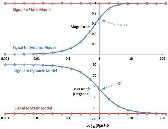


Figure 1.
The Bode plots show the magnitude and loss angle of the transfer functions over a range of operating frequencies:
  • The top figure plots the magnitude of the transfer function against Log10(ω/R) MathType@MTEF@5@5@+=feaagKart1ev2aaatCvAUfeBSjuyZL2yd9gzLbvyNv2CaerbuLwBLnhiov2DGi1BTfMBaeXatLxBI9gBaerbd9wDYLwzYbItLDharqqtubsr4rNCHbGeaGqiVu0Je9sqqrpepC0xbbL8F4rqqrFfpeea0xe9Lq=Jc9vqaqpepm0xbba9pwe9Q8fs0=yqaqpepae9pg0FirpepeKkFr0xfr=xfr=xb9adbaqaaeGaciGaaiaabeqaamaabaabaaGcbaGaaeitaiaab+gacaqGNbWaaSbaaSqaaiaaigdacaaIWaaabeaakmaabmaabaGaeqyYdCNaai4laiaadkfaaiaawIcacaGLPaaaaaa@3F2C@ .
  • The bottom figure plots the loss angle of the transfer function against Log10(ω/R) MathType@MTEF@5@5@+=feaagKart1ev2aaatCvAUfeBSjuyZL2yd9gzLbvyNv2CaerbuLwBLnhiov2DGi1BTfMBaeXatLxBI9gBaerbd9wDYLwzYbItLDharqqtubsr4rNCHbGeaGqiVu0Je9sqqrpepC0xbbL8F4rqqrFfpeea0xe9Lq=Jc9vqaqpepm0xbba9pwe9Q8fs0=yqaqpepae9pg0FirpepeKkFr0xfr=xfr=xb9adbaqaaeGaciGaaiaabeqaamaabaabaaGcbaGaaeitaiaab+gacaqGNbWaaSbaaSqaaiaaigdacaaIWaaabeaakmaabmaabaGaeqyYdCNaai4laiaadkfaaiaawIcacaGLPaaaaaa@3F2C@ .
  • Plots of the signal sent to the dynamic model are gray-blue.
  • Plots of the signal sent to the static model are brick-red.

The log scale used for the x-axis lets you view a wide range of frequencies and filter behavior as follows:

  1. When (ω/R) MathType@MTEF@5@5@+=feaagKart1ev2aaatCvAUfeBSjuyZL2yd9gzLbvyNv2CaerbuLwBLnhiov2DGi1BTfMBaeXatLxBI9gBaerbd9wDYLwzYbItLDharqqtubsr4rNCHbGeaGqiVu0Je9sqqrpepC0xbbL8F4rqqrFfpeea0xe9Lq=Jc9vqaqpepm0xbba9pwe9Q8fs0=yqaqpepae9pg0FirpepeKkFr0xfr=xfr=xb9adbaqaaeGaciGaaiaabeqaamaabaabaaGcbaWaaeWaaeaacqaHjpWDcaGGVaGaamOuaaGaayjkaiaawMcaaaaa@3AD6@ ≪ 1, that is at low frequencies, then:
    • The magnitude of the signal sent to the dynamic model is close to 0.
    • The loss angle of the signal sent to the dynamic model is close to 90°.
    • The magnitude of the signal sent to the static model is 1.
    • The loss angle of the signal sent to the static model is 0°.

    The bushing essentially behaves as the static model. The loss angle of the signal sent to the dynamic model is close to 90°, but this is not important since the magnitude of the signal is close to zero.

  2. When (ω/R) MathType@MTEF@5@5@+=feaagKart1ev2aaatCvAUfeBSjuyZL2yd9gzLbvyNv2CaerbuLwBLnhiov2DGi1BTfMBaeXatLxBI9gBaerbd9wDYLwzYbItLDharqqtubsr4rNCHbGeaGqiVu0Je9sqqrpepC0xbbL8F4rqqrFfpeea0xe9Lq=Jc9vqaqpepm0xbba9pwe9Q8fs0=yqaqpepae9pg0FirpepeKkFr0xfr=xfr=xb9adbaqaaeGaciGaaiaabeqaamaabaabaaGcbaWaaeWaaeaacqaHjpWDcaGGVaGaamOuaaGaayjkaiaawMcaaaaa@3AD6@ ≫ 1, that is at high frequencies, then:
    • The magnitude of the signal sent to the dynamic model is close to 1.
    • The loss angle of the signal sent to the dynamic model is close to 0° .
    • The magnitude of the signal sent to the static model is 1.
    • The loss angle of the signal sent to the static model is 0°.

    The bushing essentially behaves as a dynamic model superimposed on top of a static model.

  3. When (ω/R) MathType@MTEF@5@5@+=feaagKart1ev2aaatCvAUfeBSjuyZL2yd9gzLbvyNv2CaerbuLwBLnhiov2DGi1BTfMBaeXatLxBI9gBaerbd9wDYLwzYbItLDharqqtubsr4rNCHbGeaGqiVu0Je9sqqrpepC0xbbL8F4rqqrFfpeea0xe9Lq=Jc9vqaqpepm0xbba9pwe9Q8fs0=yqaqpepae9pg0FirpepeKkFr0xfr=xfr=xb9adbaqaaeGaciGaaiaabeqaamaabaabaaGcbaWaaeWaaeaacqaHjpWDcaGGVaGaamOuaaGaayjkaiaawMcaaaaa@3AD6@ ≫ 1, that is at cut-off frequency, then:
    • The magnitude of the signal sent to the dynamic model is 1/20.701 MathType@MTEF@5@5@+=feaagKart1ev2aaatCvAUfeBSjuyZL2yd9gzLbvyNv2CaerbuLwBLnhiov2DGi1BTfMBaeXatLxBI9gBaerbd9wDYLwzYbItLDharqqtubsr4rNCHbGeaGqiVu0Je9sqqrpepC0xbbL8F4rqqrFfpeea0xe9Lq=Jc9vqaqpepm0xbba9pwe9Q8fs0=yqaqpepae9pg0FirpepeKkFr0xfr=xfr=xb9adbaqaaeGaciGaaiaabeqaamaabaabaaGcbaGaaGymaiaac+cadaGcaaqaaiaaikdaaSqabaGccqGHijYUcaaIWaGaaiOlaiaaiEdacaaIWaGaaGymaaaa@3D98@ .
    • The loss angle of the signal sent to the dynamic model is 45°.
    • The magnitude of the signal sent to the static model is 1.
    • The loss angle of the signal sent to the static model is 0°.

    The bushing essentially behaves as a dynamic model superimposed on top of a static model.