After loading a file, select a method to display the participation data.
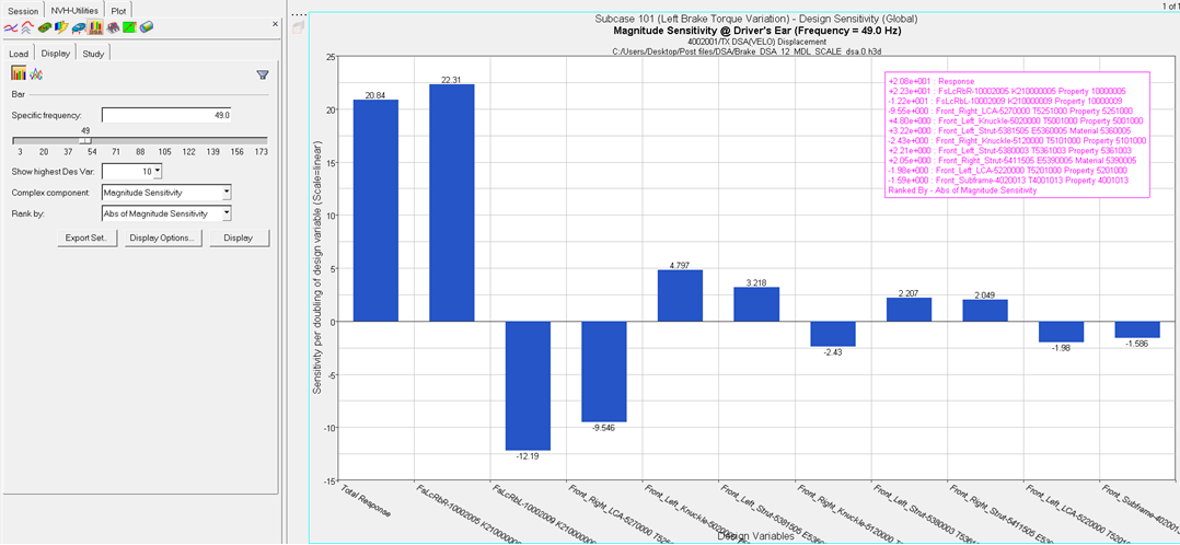
Bar
Allows you to plot design sensitivity to an acoustic or structural
response on a bar chart.
Enter a specific frequency in the Specific frequency field, or use the
slider bar to select a frequency value. When you use the slider bar to
select a frequency, a red line is displayed on the response plot and is
dragged simultaneously as you drag the slider bar.
Show highest Des Var
Select the highest number of design variables to
display.
Complex component
Magnitude Sensitivity - Plots the scalar sensitivity based
on response magnitude change. Positive values indicate that
response magnitude increases with increase in design
variable and negative values indicate that response
magnitude decreases with increase in design variable.
Projected Sensitivity - Plots scalar sensitivity values
after projecting complex design sensitivity vector to the
response. Positive values indicate that the response
magnitude increases with an increase in design variables and
negative values indicate that response magnitude decreases
with an increase in design variables.
Rank by
Abs of Projected - Design variables are ranked by the area
under the curve of the absolute values of their sensitivity
projected to the response.
Abs of Magnitude Sensitivity - Design variables are ranked
by the area under the curve of the absolute values of the
magnitude sensitivity.
Export Set
Allows you to export a .csv file
containing a design variable set definition of the top
ranked design variables.
Display Options
Customize the plot, including scale, weighting, and the plot
layout.
Display
Click Display to display the response
plot.
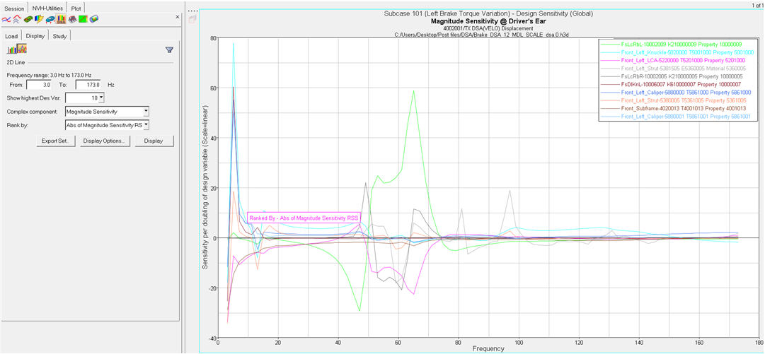
2D Line
Creates a plot of design sensitivity to an acoustic or structural
response on a 2D line plot (overlay).
Frequency range indicates the available range, based on your
dsa.0.h3d file.
Using the From and To fields to customize the frequency band.
All other options are similar to those for the Bar plot.