HM-4460: Composite
In this tutorial, you will: mesh all of the surfaces at once; define the dummy properties and assign them to the mesh; define an orientation for the component; use the Ply Realization and distribution table option; laminate realize; create and edit a distribution table; and use the Ply thickness visualization representation option.
Load the ANSYS User Profile
In this step, you will load the ANSYS user profile in HyperMesh.
- Start HyperWorks.
- From the menu bar, click .
Load the Model
In this step, you will load the model file in HyperMesh
-
In the Geometry Import Options dialog, click
Import.
Note: You will import the Ply and Composite data later in this tutorial.HyperMesh imports geometry data only.

Figure 1. -
In the Model Browser, review the model contents.

Figure 2.
Mesh all of the Surfaces at Once
In this step, you will mesh all of the model surfaces simultaneously while specifying element sizes and element types.
-
Set the elements to surf comp/elements to current comp toggle to
elems to current comp.

Figure 3. -
Click mesh.
Note: You should now be in the density subpanel of the meshing module. There is node seeding and a number on each surface edge. The number indicates the number of elements that were created along the edge.The meshing module opens.

Figure 4. -
Click return.
The mesh is accepted.

Figure 5.
Load the Ply Information from FiberSim
In this step, you will load the ply information from FiberSim in HyperMesh.
-
In the Model Browser, review the model's contents.

Figure 6. -
In the Model Browser, turn off the display of geometry for
all of the components.

Figure 7.
Review and Edit the Element Normals
In this step, you will review and edit element normals in a model in HyperMesh.
-
From the Elements ribbon, click the Normals tool.

Figure 8.Note: Element normals need to be changed to match the Z direction (red color).The Normals panel opens. -
Set the first switch to elems as seen in Figure 9.

Figure 9. -
Click display.
Note: The red side of the elements is the positive normal direction Z, while the blue side is the negative normal direction.HyperMesh displays, on each side of the part, the element normals using the colors red and blue.

Figure 10. - Optional:
If the blue color is in the Z direction, click and then click reverse.
All of the elements are set in the right normal direction (red).

Figure 11.
Realize Ply Geometry Shape
In this step, you will realize the ply geometry shape.
-
In the graphics area, click the three dots besides the components selector, as
seen in Figure 12.

Figure 12. -
In the Advanced Selection dialog, select all listed
components.

Figure 13. -
Set Search Criterion to Element centroid.

Figure 14. -
Click Realize.
This process takes each FiberSim Ply data and finds the FE elements which are bounded by the ply boundaries, and transfers the ply directions, draping data, and ply orientation into FE elements. This process also converts geometry plies into FE plies. At the end of realization, HyperMesh creates sets containing FE elements for each ply.

Figure 15.
Add an Element Type
In this step, you will add an element type.
-
In the Solver Browser, review the new element type.

Figure 16.
Define Material Properties
-
Set card image to
MATERIAL.

Figure 17. -
For MP_EX_LEN (Number of Elastic moduli to input), enter
1.

Figure 18. -
For C, enter 2.1e5.
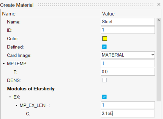
Figure 19.
Create the Section Card for the Shell Elements in the Model
-
For MAT, click .

Figure 20. -
In the new Entity Editor, change the config to
Shell, set the Tk value to
0.5, then click Previous.

Figure 21. -
Click the search icon then assign sensor1.

Figure 22.
Update the Component with Property
In this step, you will update the component with the SECTYPE property.
Ply Visualization
In this step you will verify FE plies thickness and orientation in HyperMesh.
-
Set the entity selector in the graphics area to
Properties.

Figure 23.This automatically colors faces based on their associated properties. -
On the View Controls toolbar, click
 .
.
-
Set the layer representation mode to Ply layers and
direction.

Figure 24. -
In the Model Browser, Hide and
Show each Ply.

Figure 25.
Figure 26.
Laminate Realize the Ply Based Model
In this step, you will laminate realize the ply-based model.
-
In the Laminate Realize dialog, accept the default
settings and click Realize.

Figure 27.HyperMesh creates a property for each stack, and assigns it to a component. -
Set the entity selector in the graphics area to
Components to change the face coloring.
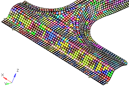
Figure 28.
Export the Deck to ANSYS *.cdb Format
In this step, you will export the deck to ANSYS *.cdb format.