Create a Forming Limit Diagram Plot

Once a forming limit curve is defined, you can use it to plot a forming limit diagram and formability contours on a deformable material using the FLD tab.
  1. From the Load Model panel, load a simulation.
  2. Go to the FLD panel.
  3. From the study list, select the study to be used for the current plot.
  4. Click the FLD tab.


    Figure 1. FLD Tab
  5. Define the metric for the FLD using the Type drop-down menu:
    • True Strain
    • Engineering Strain
    By default it is assigned the metric of the input FLC curve, however you can change the type at any instance by clicking Apply (the metric of FLD will then be updated along with data points and the FLC curve to the corresponding metric).
  6. Select one or more components to be used for the FLD plot.
    • Click the Components input collector and use the extended entity selection menu.
    • Pick entities directly from the model in the modeling window.
    Note: If no selection is made, all of the components will be used to create an FLD plot.
  7. Select Strain as the result type.
  8. Select an element layer at which the FLD is being created using the second drop-down menu in the Result Type section.
  9. For Display, select a contour.
    • Zone contour - creates a formability contour based on the deformation mode, which is derived from the ratio of major and minor strains.
    • Distance contour - creates a formability contour based on the distance of each strain pair from the FLC.
    • Failure contour (%) - Creates a failure contour based on the relative distance of an element in FLC from line (Y1/Y2)*100. See the figure below. Its value will be between 0-100 for points below the failure line and above 100 for points above the failure line.


      Figure 2.
  10. Activate the Shear line check box.
  11. Select an option from the Shear line drop-down menu.
    • Use Angle - set the angle of the Shear line with respect to the minor strain axis. 45 degrees is the default angle. This definition is always in a True Strain metric; HyperView will automatically convert them if the FLD Type is set to Engineering Strain.
    • Use file - select a file which contains the Shear line data in xy format. The metric of data needs to be specified at the start of file as either Engineering Strain or True Strain. If no metric is provided, then the data is assumed to be of a True Strain metric.
  12. Activate the Margin line offset (%) check box.
  13. Select an option from the Margin line offset (%) drop-down menu.
    • Absolute - the margin line is obtained by offsetting the FLC curve down by a constant value. The constant value is input as a percentage. This will result in the margin line approximately parallel to FLC curve.
    • Relative - the margin line is obtained by offsetting each point of the FLC curve down by a multiple of its value. The multiple is input as a percentage. This will result in the margin line diverging from FLC curve.
  14. Activate the Uniaxial compression line check box. and enter an R Value or Use Angle value.
  15. Select an option from the Uniaxial compression line drop-down menu.
    • R Value - the uniaxial compression line is obtained from normal anisotropy of the material.
    • Use Angle - set the angle of the uniaxial compression line with respect to the minor strain axis (26.57 degrees is the default angle). This definition is always in a True Strain metric; HyperView will automatically convert them if the FLD Type is set to Engineering Strain.
  16. Activate the Loose metal bound (%) check box and enter a percentage value.
    A semi-circle around the origin with 2% strain as the default radius. The percentage is always in a Engineering Strain metric; HyperView will automatically convert them if the FLD Type is set to True Strain.
  17. Activate the Fit curve (FLC) check box.
    This will create a curve fit through the given set of points for the FLC corresponding to the File and Values methods.
  18. Click Apply.
    Tip: The 2D window showing the FLD plot displays the chosen FLC curve. If you select a different curve, the plot can be updated to reflect that graph by clicking Apply.
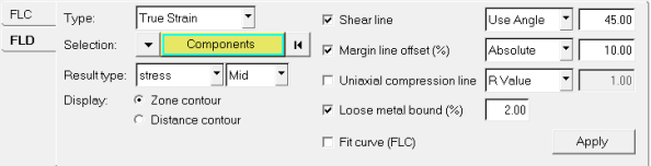
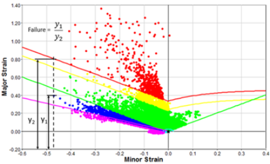
    The forming limit diagram plot is displayed showing the minor strain and major strains or stresses along the x and y axes (respectively) in the same plot as the forming limit curve. The FLD automatically plots the marginal FLC, the loose metal bound, and lines at ±45 degrees with respect to the major axis. The elements in the model in the main 3D window change color to create a formability contour based on the corresponding colors in the FLC. The color scheme is:
    Red
    Failure (points above the FLC)
    Yellow
    Marginal (points between the FLC and safety curve)
    Green
    Safe (Points between ± 45 degree line and safety curve)
    Blue
    Compression (Points to the left of -45 degree line)
    Light Blue
    Loose metal (Points within a radius of 2% major or minor strain)
    Note: The 3D window also displays a legend using the color distribution above. The legend properties can be changed by clicking Edit Legend.
    Tip: The formability contours can be animated by clicking the start/pause transient animation icon.
    You can also mask simulation data so that only the FLD corresponding to the displayed component (part) of the FE model are displayed.
  19. Use Circle Zoom to zoom in on a set of points on the FLD plot.
    The points inside the zoom box fill the 2D window.
    Note: Click the Fit icon to re-plot all the strain points.