Example 13: Boat MOM-GTD

This case explains how to use the Dolph-Chebychev algorithms to calculates the pointing parameters in a bidimensional coaxial feed array, and how to use the resulting radiation pattern in physical applications.

Step 1 Create a new MoM Project.

Open newFASANT and select File - New option.

Figure 1. New Project panel

Select MOM option on the previous figure and start to configure the project.

Step 2 Set the simulation parameters as shown.

Select Simulation - Parameters option, set the parameters and save it.

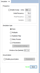
Figure 2. Simulation panel

Step 3 Create the array

First, select 'millimeters' on units list on the bar at the bottom of the main window.

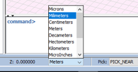
Figure 3. The first element is created using Source - Coaxial Feed - Add Feed Point.

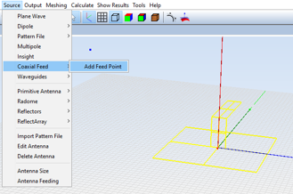
Figure 4. Add feed point

Select the surfaces and click on Add.

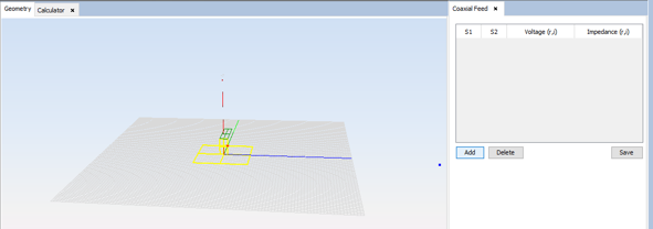
Figure 5. Coaxial Feed panel

Then save the feed point.

Use the array command and enter the characteristics of the array.

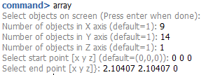
Figure 6. Array parameters

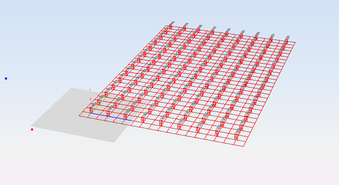
Figure 7. Array view

Step 4 Feed the array

To set the feeding of the array select Source - Antenna Feeding and the following panel will open.

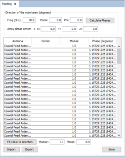
Figure 8. Antenna Feeding panel

This is the default setting. To use the Dolph-Chebychev algorithm click on Tools - User Function and select the corresponding function. NOTE To use the bidimensional Dolph-Chebychev function it is needed to download both the bidimensional and the unidimensional functions.

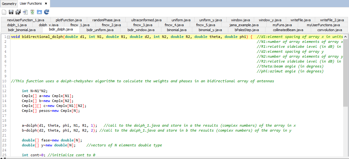
Figure 9. Bidimensional Dolph-Chebychev function

A path has been selected by default so the files will be created on the mydatafiles folder in the newFASANT directory.

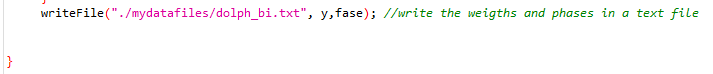
Figure 10. Bidimensional Dolph-Chebychev function

The next step is generating the text file. To do so click on Tools - Calculator and write the call to the function.

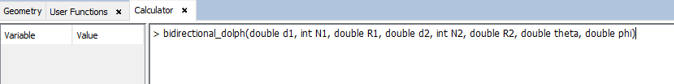
Figure 11. Calculator panel

In this case, set the parameters as shown. Angles of theta=0º and phi=0º, and a sidelobe level of 50 dB are selected as an example.

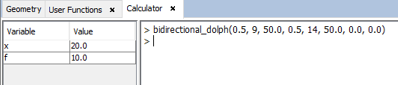
Figure 12. Calculator panel

A spacing of 0.5 in units of lambdas is selected because is equivalent to a spacing of 2.104 millimeters at 70 GHz.

The text file will be automatically generated in the mydatafiles folder.

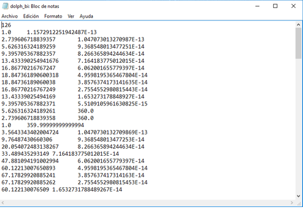
Figure 13. Results file

Now, apply these results to the array created before by clicking on Source - Antenna Feeding.

The panel shown before will appear. To use the weights and phases calculated with the Dolph-Chebychev algorithm, click on Import.

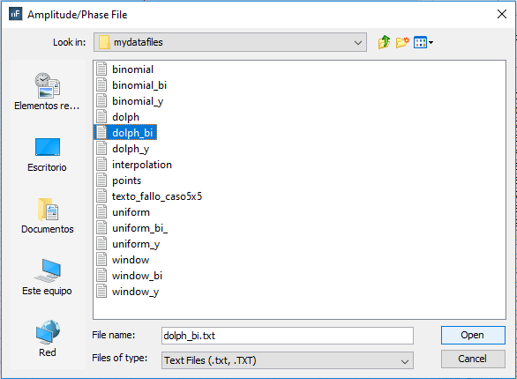
Figure 14. Amplitude/Phase File panel

Select the corresponding file and save the feeding.

Step 5 Solver parameters

Select Solver - Advanced Options and set the parameters as shown.

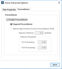
Figure 15. Solver Advanced Options panel

Step 6 Meshing the geometry model.

Select Mesh - Create Mesh to open the meshing configuration panel and then set the parameters as show the next figure.

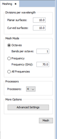
Figure 16. Meshing panel

Step 7 Execute the simulation.

Select Calculate - Execute option to open simulation panel.

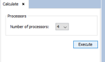
Figure 17. Calculate panel

Step 8 Show Results

The radiation cuts can be visualized by clicking on Show Results - Radiation Pattern - View Cuts.

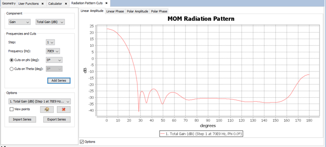
Figure 18. Radiation Pattern Cuts

Note that the side lobe level selected earlier must be represented here.

The radiation pattern can be visualized by clicking on Show Results - Radiation Pattern - View 3D Pattern.

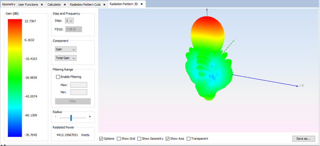
Figure 19. Radiation Pattern 3D

Step 9 Rotate the array

In order to obtain the radiation in the desired orientation, rotate the array.

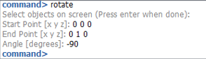
Figure 20. Rotate parameters

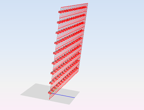
Figure 21. Array view

Step 10 Obtain results

Now, mesh and execute the case again. The desired results are as shown.

NOTE to visualize the polar amplitude, click on Show Results - Radiation Pattern - View Cuts and then select Polar Amplitude.

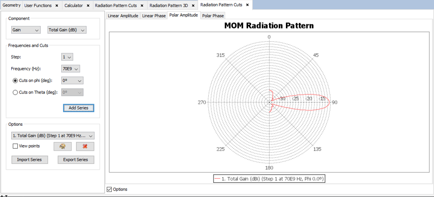
Figure 22. Radiation Pattern Cuts

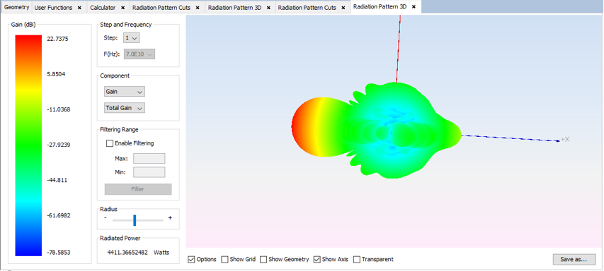
Figure 23. Radiation Pattern 3D

Step 10 Export results

Export these results by clicking on Show Results - Radiation Pattern - Export as DIA File.

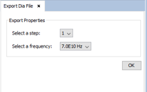
Figure 24. Export DIA File panel

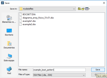
Figure 25. Create the file and click on Save. To complete this action, click on OK.

Now, save the project and exit it.

Step 11 Create a GTD project

Create a new project, this time with the GTD module.

Figure 26. New Project panel

Step 12 Create the geometry

First, add the boat to the project, by clicking on Geometry - Import.

Select the corresponding .igs file and open it.

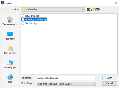
Figure 27. Open file panel

Rotate the ship so it is aligned with the radiation direction.

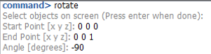
Figure 28. Rotate parameters

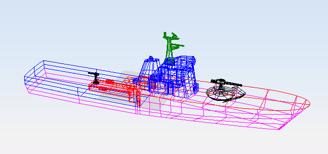
Figure 29. Boat view

To introduce the desired radiation pattern into the project, click on Antenna - Import DIA File.

Select the .dia file created earlier in the MoM project and open it.

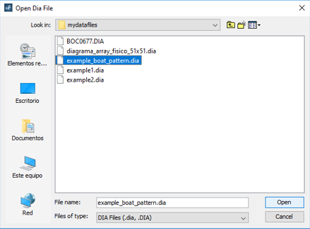
Figure 30. Open DIA File panel

To add the antenna to the project, click on Antenna - Pattern File Antenna - Pattern File Antenna. Add the .dia file and create a dipole antenna with the parameters shown below.

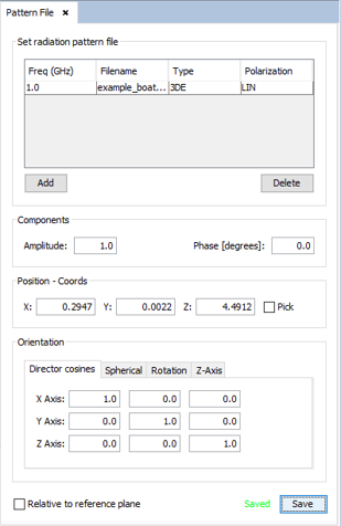
Figure 31. Pattern File panel

Step 13 Set the simulation parameters as shown.

Select Simulation - Parameters option, set the parameters and save it.

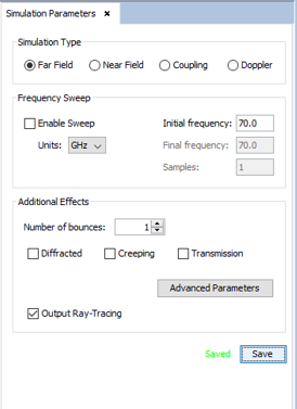
Figure 32. Simulation Parameters panel

Step 14 Observation directions

Click on Observation Directions.

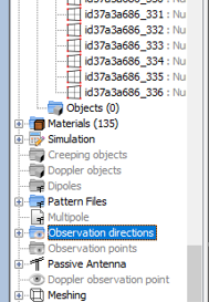
Figure 33. Set the parameters as shown.

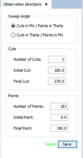
Figure 34. Observation Directions panel

Step 15 Meshing the geometry model.

Select Meshing - Create Visibility Matrix to open the meshing configuration panel and then set the parameters as show the next figure.

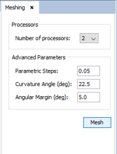
Figure 35. Meshing panel

Step 16 Execute the simulation.

Select Calculate - Execute option to open simulation panel.

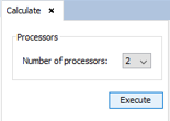
Figure 36. Calculate panel

Step 17 Show Results

To visualize the rays from the antenna, click on Show Results - View Ray.

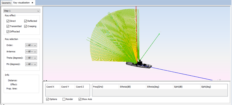
Figure 37. Ray Visualization

Figure 38. Ray Visualization

The radiation cuts can be visualized by clicking on Show Results - Far Field - View Cuts. NOTE to visualize the polar amplitude, click on Polar Amplitude.

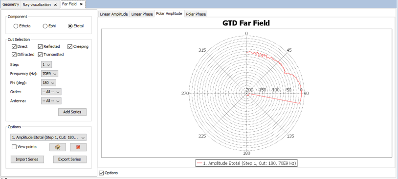
Figure 39. Far Field Cuts

Here is a comparison of this example with a project that has the same antenna but without the boat. The blue line represents the array with the boat and the red line is the project without the boat.

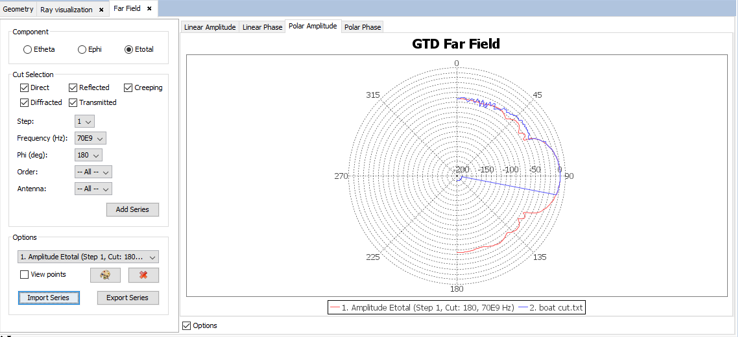
Figure 40. Far Field Cuts