/MAT/LAW110 (VEGTER)

#RADIOSS STARTER
#---1----|----2----|----3----|----4----|----5----|----6----|----7----|----8----|----9----|---10----|
/UNIT/25
Local unit system
                  Mg                  mm                   s
#---1----|----2----|----3----|----4----|----5----|----6----|----7----|----8----|----9----|---10----|
#-  2. MATERIALS:
#---1----|----2----|----3----|----4----|----5----|----6----|----7----|----8----|----9----|---10----|
/MAT/LAW110/1/25
Steel: Icrit = 1, example with 3 angles (0°, 45° and 90° to the RD)
#        Init. dens.
             7.85E-9
#                  E                  nu
            194200.0                 0.3
#---1----|----2----|----3----|----4----|----5----|----6----|----7----|----8----|----9----|---10----|
#    Icrit   TAB_YLD          MAT_Xscale          MAT_Yscale                 fBI               rhoBI            
         1         0                 0.0                 0.0               1.004               0.889                         
#               YLD0               DSIGM                BETA               OMEGA                   n
               107.1               179.6                0.25                8.07                 1.0
#               EPS0                SIGS                 DG0               Deps0                   m
                 0.0                20.0                 800             3.61e-3                 1.0
#               TINI              C_HARD               F_CUT        VP   Ismooth  TAB_TEMP
               293.0                 0.0             10000.0         1         1         0
#          fUN_THETA             R_THETA          fPS1_THETA          fPS2_THETA           fSH_THETA 
               1.021                0.64               1.061              0.5305               0.560
               0.987                0.48               1.037              0.5185               0.640 
               1.009                0.76               1.048              0.5240               0.560 
#---1----|----2----|----3----|----4----|----5----|----6----|----7----|----8----|----9----|---10----|
#---1----|----2----|----3----|----4----|----5----|----6----|----7----|----8----|----9----|---10----|
/MAT/LAW110/2/25
Steel :Icrit = 2, example with 3 angles (0°, 45° and 90° to the RD)
#        Init. dens.
             7.85E-9
#                  E                  nu
            194200.0                 0.3
#---1----|----2----|----3----|----4----|----5----|----6----|----7----|----8----|----9----|---10----|
#    Icrit   TAB_YLD          MAT_Xscale          MAT_Yscale                 fBI               rhoBI            
         2         0                 0.0                 0.0               1.004               0.889                         
#               YLD0               DSIGM                BETA               OMEGA                   n
               107.1               179.6                0.25                8.07                 1.0
#               EPS0                SIGS                 DG0               Deps0                   m
                 0.0                20.0                 800             3.61e-3                 1.0
#               TINI              C_HARD               F_CUT        VP   Ismooth  TAB_TEMP
               293.0                 0.0             10000.0         1         1         0
#          fUN_THETA             R_THETA          fPS1_THETA          ALPS_THETA           fSH_THETA 
               1.021                0.64               1.061                 0.5               0.560
               0.987                0.48               1.037                 0.5               0.640 
               1.009                0.76               1.048                 0.5               0.560 
#---1----|----2----|----3----|----4----|----5----|----6----|----7----|----8----|----9----|---10----|
#---1----|----2----|----3----|----4----|----5----|----6----|----7----|----8----|----9----|---10----|
/MAT/LAW110/3/25
Steel
#        Init. dens.
             7.85E-9
#                  E                  nu
            194200.0                 0.3
#---1----|----2----|----3----|----4----|----5----|----6----|----7----|----8----|----9----|---10----|
#    Icrit   TAB_YLD          MAT_Xscale          MAT_Yscale                 fBI               rhoBI            
         3         0                 0.0                 0.0               1.004               0.889                         
#               YLD0               DSIGM                BETA               OMEGA                   n
               107.1               179.6                0.25                8.07                 1.0
#               EPS0                SIGS                 DG0               Deps0                   m
                 0.0                20.0                 800             3.61e-3                 1.0
#               TINI              C_HARD               F_CUT        VP   Ismooth  TAB_TEMP
               293.0                 0.0             10000.0         1         1         0
#               RM_0               RM_45               RM_90                AG_0               AG_45
               408.4               408.4               408.4                20.0                20.0
#              AG_90                 R_0                R_45                R_90
                20.0                0.64                0.48                0.76    
#---1----|----2----|----3----|----4----|----5----|----6----|----7----|----8----|----9----|---10----|
#---1----|----2----|----3----|----4----|----5----|----6----|----7----|----8----|----9----|---10----|
/MAT/LAW110/4/25
Steel :example with 3 angles (0°, 45° and 90° to the RD)
#        Init. dens.
             7.85E-9
#                  E                  nu
            194200.0                 0.3
#---1----|----2----|----3----|----4----|----5----|----6----|----7----|----8----|----9----|---10----|
#    Icrit   TAB_YLD          MAT_Xscale          MAT_Yscale                 fBI               rhoBI            
         4         0                 0.0                 0.0               1.004               0.889                         
#               YLD0               DSIGM                BETA               OMEGA                   n
               107.1               179.6                0.25                8.07                 1.0
#               EPS0                SIGS                 DG0               Deps0                   m
                 0.0                20.0                 800             3.61e-3                 1.0
#               TINI              C_HARD               F_CUT        VP   Ismooth  TAB_TEMP
               293.0                 0.0             10000.0         1         1         0
#          fUN_THETA             R_THETA                W_PS                W_SH
               1.021                0.64              0.4125                0.75
               0.987                0.48              0.4125                0.75
               1.009                0.76              0.4125                0.75 
#---1----|----2----|----3----|----4----|----5----|----6----|----7----|----8----|----9----|---10----|
#enddata

1. If $I_{crit}$ = 1, the law uses the classic Vegter yield criterion which is defined by:
   (1)

   $$\varphi =\overline{\sigma }-{\sigma }_Y$$
   Where,

   $\varphi$

   Yield function.

   ${\sigma }_Y$

   Yield stress.

   $\overline{\sigma }$

   Interpolated Vegter equivalent stress.

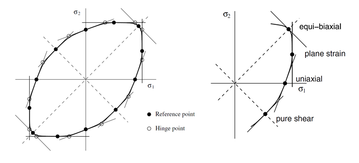
   The Vegter yield locus, under plane stress conditions, is obtained by defining three second order Bezier interpolation curves in the principal stresses space (Figure 1).

   
   
   Figure 1. Yield criterion defined by the classic Vegter formulation in plane-stress (I_crit=1)

   These curves are used to link four reference points which are measured experimentally at different loading conditions: shear, uniaxial tension, plane strain, and equibiaxial tension. Between two reference points, the yield locus is then defined in:(2)

   $$\sigma = \left(\begin{array}{c}{\sigma }_1\\ {\sigma }_2\end{array}\right) = \overline{\sigma }\left(\begin{array}{c}{f}_1\\ f_2\end{array}\right) = \left(\begin{array}{c}{\sigma }_1^{r1}\\ {\sigma }_2^{r1}\end{array}\right)+2\mu \left(\begin{array}{c}{\sigma }_1^{r1}-{\sigma }_1^h\\ {\sigma }_2^{r1}- {\sigma }_2^h\end{array}\right)+{\mu }^2\left(\begin{array}{c}{\sigma }_1^{r2}+ {\sigma }_1^{r1}-2{\sigma }_1^h\\ {\sigma }_2^{r2}+ {\sigma }_2^{r1}- 2{\sigma }_2^h\end{array}\right)$$
   Where,

   ${\sigma }^{r1}$ , ${\sigma }^{r2}$

   Two reference points.

   ${\sigma }^h$

   Hinge point, which is computed automatically.

   $\mu$

   Parameter computed at each time step to determine the position on the yield locus.

   The four measured reference points are referred to as: $f_{sh}$ , $f_{un}$ , $f_{ps}$ , and ${ƒ}_{bi}$ . The coordinates of these reference points are provided by you.

   Where, $f_{sh}^2$ = $-f_{sh}^1= -f_{sh}$ , $f_{un}^2=0$ , $f_{bi}^2= f_{bi}^1=f_{bi}$ . For a given direction with respect to the rolling direction, only one component must be set for the shear $f_{sh}$ , uniaxial tension $f_{un}$ , and equibiaxial tension reference point ${ƒ}_{bi}$ . For the plane-strain reference point, the two components $f_{ps}^1$ and $f_{ps}^2$ must be provided by you.

   There is a freedom on the choice of the second coordinate $f_{ps}^2$ . If it is not set, its value will be taken as an average of the second coordinates of the two neighboring hinge points.

   The hinge point located between two reference points is computed using the reference points coordinates, but also the normal to the yield surface in each reference point. Using the normality rule, the normal to the yield surface can be expressed using the strain rate tensor component:(3)

   $$n= \left(\begin{array}{c}{n}_1\\ n_2\end{array}\right)= \left(\begin{array}{c}{\dot{\epsilon }}_1\\ {\dot{\epsilon }}_2\end{array}\right)= \left(\begin{array}{c}1\\ \frac{{\dot{\epsilon }}_2}{{\dot{\epsilon }}_1}\end{array}\right)= \left(\begin{array}{c}1\\ {\rho }_r\end{array}\right)$$
   Where, ${\rho }^r$ is the strain rate ratio in a given reference point. For the shear reference point, ${\rho }_{sh}=-1$ . For the plane-strain reference point, ${\rho }_{ps}=0$ . For the uniaxial tension reference point, this ratio can be computed from the Lankford coefficient denoted $R$ :(4)

   $${\rho }_{un}= \frac{-R}{R+1}$$

   The Lankford coefficient must be provided by you. Finally, the strain rate ratio in the equibiaxial tension ${ƒ}_{bi}$ must also be set.

2. If $I_{crit}$ = 2, the standard Vegter criterion is used. It is the same criterion as the classical Vegter, with a different input card. In this card, the second coordinate of the plane strain point is computed as a weighted average of the second coordinate of the two neighboring hinge points ${\sigma }_{h1}$ and ${\sigma }_{h2}$ :
   (5)

   $$f_{ps}^2={\sigma }_{h1}^2+{\alpha }_{ps}\left({\sigma }_{h2}^2- {\sigma }_{h1}^2\right)$$
3. If $I_{crit}$ = 3, the Vegter 2017 yield criterion is used. It is the same criterion as the classical Vegter, with a different input card. In this card, all parameters are determined from the maximum uniaxial engineering stress $R_m^i$ , the maximum uniform elongation $A_g^i$ , and the Lankford coefficient $R^i$ . These three parameters must be given for three directions at an angle $i$ degrees with respect to the rolling direction RD: 0 degrees, 45 degrees, and 90 degrees. For this criterion, the number of angles is locked at 3.
4. If $I_{crit}$ = 4, the law uses the simplified Vegter Lite yield criterion which is defined by:
   (6)

   $$\varphi =\overline{\sigma }-{\sigma }_Y$$
   Where,

   $\varphi$

   Yield function.

   ${\sigma }_Y$

   Yield stress.

   $\overline{\sigma }$

   Interpolated Vegter equivalent stress.

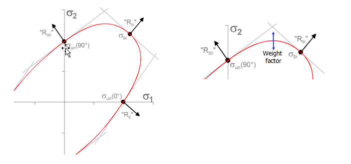
   The Vegter yield locus, under plane stress conditions, is obtained by defining two second order Nurbs interpolation curves in the principal stresses space. These curves are used to link three reference points which are measured experimentally at different loading conditions: uniaxial compression, uniaxial tension, and equibiaxial tension. Between two reference points, the yield locus is then defined in:(7)

   $$\sigma = \left(\begin{array}{c}{\sigma }_1\\ {\sigma }_2\end{array}\right) = \overline{\sigma }\left(\begin{array}{c}{f}_1\\ f_2\end{array}\right) =\frac{{\left(1-\mu \right)}^2\left(\begin{array}{c}{\sigma }_1^{r1}\\ {\sigma }_2^{r1}\end{array}\right)+2\mu \left(1-\mu \right)w_h\left(\begin{array}{c}{\sigma }_1^h\\ {\sigma }_2^h\end{array}\right)+{\mu }^2\left(\begin{array}{c}{\sigma }_1^{r2}\\ {\sigma }_2^{r2}\end{array}\right)}{{\left(1-\mu \right)}^2+2\mu \left(1-\mu \right)w_h+ {\mu }^2 }$$

   (8)

   $$0\le \mu \le 1,w_h\ge \text{0}$$
   Where,

   ${\sigma }^{r1}$ , ${\sigma }^{r2}$

   Two reference points.

   ${\sigma }^h$

   Hinge point, which is computed automatically.

   $\mu$

   Parameter computed at each time step to determine the position on the yield locus.

   $w_h$

   Weight factor associated with the hinge point.

   
   
   Figure 2. Yield criterion defined by the classic Vegter formulation in plane-stress (I_crit=2)

   In Figure 2, yield criterion is defined by the classic Vegter formulation in plane-stress ( $I_{crit}$ = 2).

   As for the classical Vegter formulation, you must set the parameters $f_{un}$ , ${ƒ}_{bi}$ , $R$ , and ${\rho }_{bi}$ . In this simplified formulation, the two hinge points are in pure shear and plane strain condition. The two associated weight factors $w_{sh}$ and $w_{ps}$ must also be defined.

5. To take into account the anisotropy, you can define a set of parameters for several $N_{angle}$ directions at different angle $\varphi$ with respect to the rolling direction RD. These directions must be equally distributed between 0 and $\frac{\pi }{2}$ . For all loading directions that are located between the given directions, the Vegter model proposes to use a Fourier series interpolation.
   Not all parameters must be defined for each direction. The parameter ${ƒ}_{bi}$ is uniform among all the directions. The strain rate ratio ${\rho }_{bi}$ in the direction 0 (rolling direction) is sufficient to determine this ratio for all other directions:(9)

   $${\rho }_{bi}\left(\theta \right)= \frac{\left({\rho }_{bi}+1\right)+\left({\rho }_{bi}-1\right)\cos 2\theta }{\left({\rho }_{bi}+1\right)-\left({\rho }_{bi}-1\right)\cos 2\theta }$$
   For all other parameters, the following Fourier interpolation is used:(10)

   $$f_{un}\left(\theta \right)={\displaystyle \sum }_{m=0}^{N_{angle}-1}{\text{ψ}}_{\text{un}}^m \text{cos}\left(2m\theta \right)$$
   In the case of the classic, standard, and 2017 Vegter formulation ( $I_{crit}$ = 1, 2, 3), a similar operation is used. (11)

   $$f_{sh}^2\left(\theta \right)=-f_{sh}^1 \left(\frac{\pi }{2}-\theta \right)$$
   In the case of the simplified Vegter Lite formulation ( $I_{crit}$ = 4), a similar interpolation is used on $R$ , $w_{sh}$ , and $w_{ps}$ . In this case:(12)

   $$w_{sh}\left(\theta \right)= w_{sh}\left(\frac{\pi }{2}-\theta \right)$$
6. Parameters must define a convex yield locus, otherwise the simulation might be unstable. That is why a data check is present in the Radioss Starter to check the yield criterion convexity.
7. When only one direction is defined, $N_{angle}$ = 1, the material law is isotropic and must be used with /PROP/TYPE1 (isotropic shell). If more than 1 direction is defined, $N_{angle}$ > 1 or $I_{crit}$ = 3, the material law becomes anisotropic and must be used with /PROP/TYPE9 (orthotropic shells).
8. The yield stress ${\sigma }_Y$ is defined by the following expression:
   (13)

   $${\sigma }_Y={\sigma }_0+\text{Δ}{\sigma }_m\left[\beta \left({\epsilon }_p+{\epsilon }_0\right)+{\left(1-e^{-\text{Ω}\left({\epsilon }_p+{\epsilon }_0\right)}\right)}^n\right]+{\sigma }_0^{\star }{\left[1+\frac{kT}{\text{Δ}{G}_0}\ln \left(\frac{\dot{\epsilon }}{\dot{{\epsilon }_0}}\right)\right]}^m$$
   Where,

   ${\sigma }_0$

   Initial yield stress.

   $\text{Δ} {\sigma }_m$

   Hardening stress increment.

   $\beta$

   Large strain hardening parameter.

   ${\epsilon }_0$

   Initial plastic strain.

   $\text{Ω}$

   Small strain hardening parameter.

   $\eta$

   Hardening exponent.

   ${\sigma }_0^{\star }$

   Limit dynamic flow stress.

   $k$

   Boltzmann constant.

   $T$

   Temperature.

   $\text{Δ}{G}_0$

   Maximum activation enthalpy.

   ${\dot{\epsilon }}_0$

   Inviscid limit strain rate.

   $m$

   Strain rate dependence exponent.

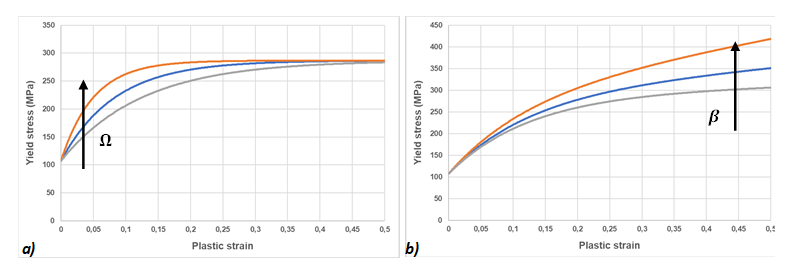
   The parameter, $\text{Ω}$ is called small strain hardening parameter, as its effect has a strong influence on the hardening curve at small strain (Figure 3a). Similarly, the large strain hardening parameter has a bigger influence at large strain (Figure 3b).

   
   
   Figure 3. Effect of hardening parameter on the yield stress evaluation

9. If T_ini is defined, the temperature will be constant at the T_ini value over the simulation. This will enable a constant strain rate dependency (Figure 4a).
   If you want to compute a temperature evolution to take into account the thermal activation effect (slight increase of strain rate dependency following the increase of the temperature), the option /HEAT/MAT must be defined (Figure 4a).

   
   
   Figure 4. Effect of temperature setting on the strain rate dependency

10. The strain rate $\dot{\epsilon }$ computation depends on the value of the flag $VP$ :
    • If $VP$ = 1: the plastic strain rate is used.
    • If $VP$ = 2: the total strain rate is used.
    • If $VP$ = 3: the deviatoric strain rate is used.
    In all cases the strain rate computation includes a filtering, using the cutting off frequency $F_{cut}$ , which is user-defined, such that:(14)

    $${\dot{\epsilon }}_f=\alpha {\dot{\epsilon }}^n+\left(1-\alpha \right){\dot{\epsilon }}^{n-1}$$

    With $\alpha = 2\pi F_{cut} \text{Δ}t$ .

11. If you want to use a tabulated hardening yield stress, the ID of the tabulated function TAB_YLD must be defined. This table can be used to define several yield stress evolutions with the plastic strain, at several strain rates. Two scale factor can be also defined in the X and Y directions. In this case, the hardening parameters ${\sigma }_0$ , $\text{Δ} {\sigma }_m$ , $\beta$ , $\text{Ω}$ , and $\eta$ are ignored, and the yield stress becomes:(15)
    $${\sigma }_Y={\text{f}}_{\text{Y}}\left({\epsilon }_{\text{p}},\dot{\epsilon }\right)$$
    Furthermore, you can also define a tabulated yield stress with plastic strain and temperature TAB_TEMP, to consider the thermal softening in adiabatic condition. In this case, the yield stress becomes:(16)

    $${\sigma }_Y={\text{f}}_{\text{Y}}\left({\epsilon }_{\text{p}},\dot{\epsilon }\right)\frac{{\text{f}}_{\text{temp}}\left({\epsilon }_{\text{p}},\text{T}\right)}{{\text{f}}_{\text{temp}}\left({\epsilon }_{\text{p}},{\text{T}}_{\text{ini}}\right)}$$
    Where,

    T_ini

    Reference temperature.

    $T$

    Actual temperature computed using the /HEAT/MAT option.

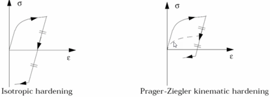
12. You might also want to use a kinematic hardening by setting coefficient C_hard:
    • If C_hard = 0: the isotropic hardening is used.
    • If C_hard = 1: the Prager-Ziegler kinematic hardening is used.
    • If 0 ≤ C_hard ≤ 1: the model is interpolated between the isotropic and the kinematic hardening.

      
      
      Figure 5.