Tutorial: Co-Simulation with MotionSolve
Learn how to build a Multi-Body System Model (MBS) of an inverted pendulum, combine it with a controls system model, and co-simulate the models.
Files for This Tutorial
Inverted_Pendulum_Tutorial.scm; Inverted_Pendulum_Tutorial.mdl
Overview of Co-Simulation and Prerequisites
Co-simulation enables MotionSolve Multi-Body Dynamics (MBS) models and Activate models to communicate with each other during simulation.
An ideal use case for co-simulation is the development of a control system for an MBS model. This tutorial shows you how to develop such a control system for an inverted pendulum.
An inverted pendulum is a pendulum that has its center of mass above its pivot point, such as a pendulum moving horizontally with its pivot point mounted on a moving railroad cart. Whereas a normal pendulum is stable when hanging downward, an inverted pendulum is inherently unstable, and must be actively balanced in order to remain upright either by applying a torque at the pivot point or by moving the pivot point horizontally as part of a feedback system.
This tutorial shows you how to design a control force acting horizontally on a cart to keep a pendulum upright, much like a child balancing a stick on his hand. The inverted pendulum is a classic problem in dynamics and control theory and is used as a benchmark for testing control strategies. Some real-world examples of inverted pendulum problems include attitude control of a rocket at launch, and the balance and movement of a Segway motorized vehicle.
Prerequisites
The installation of HyperWorks MotionSolve software is required for co-simulation. MotionSolve offers powerful modeling, analysis, visualization and optimization capabilities for multi-disciplinary simulations that include kinematics and dynamics, statics and quasi-statics, linear and vibration studies, stress and durability, loads extraction, co-simulation, effort estimation, and packaging synthesis.
Defining the Software Path Settings
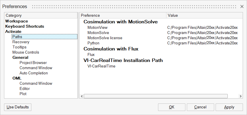
Defining the paths to MotionSolve and other software that is required for local and remote co-simulation methods.
-
On the left column of the dialog, select the category, Activate
Paths.
Building an Inverted Pendulum
Build a Multi-Body System (MBD) model of an inverted pendulum on a cart.
Entities in the MBS Model
- Pendulum
- Cart
- Rod to connect the pendulum to the cart
- Rail on which the cart is constrained to move horizontally
- Pivot which is located on the cart, between the pendulum and cart
Building the Geometry
With MotionView software, create the geometry for the inverted pendulum.
Adding Bodies
Add the pendulum and cart to your model.
Adding Joints
Add a revolute and translational joint to the model.
-
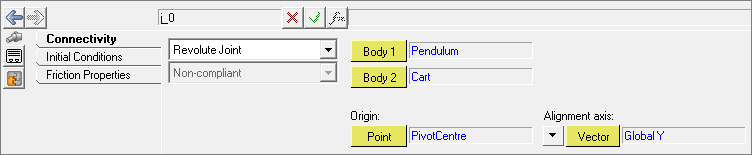
Insert a revolute joint, label it PendulumPivot, and
set the Connectivity parameters as follows:
-
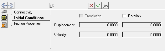
Set the Initial Conditions as follows:
-
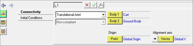
Insert a translational joint, label it CartTranslation,
and set the Connectivity parameters as follows:
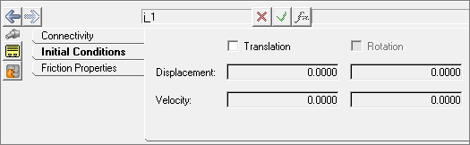
-
Set the Initial Conditions as follows:
Adding Graphics
Graphics are essential for understanding the model behavior in an animation.
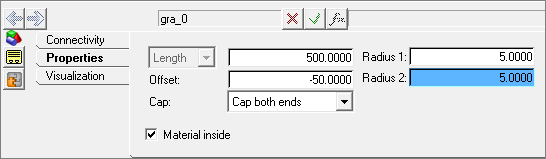
-
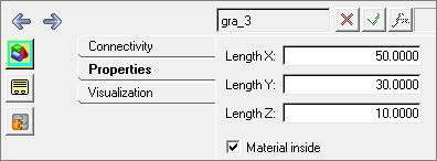
Set the Properties as follows:
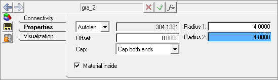
-
Set the Properties as follows:
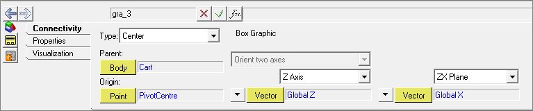
-
For Connectivity parameters, set the Type to Center; set
the Parent Body to Cart; set the Origin Point to
PivotCenter; set the Z axis direction to Vector
Global Z; set the ZX plane direction to Vector
Global X.
-
Set the Properties as follows:
Adding Forces
Apply translational forces to the Cart.
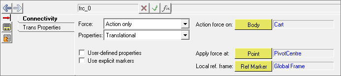
-
On the Connectivity tab, add the force, frc_0, label it
Control Force, and set the Connectivity properties as
follows:
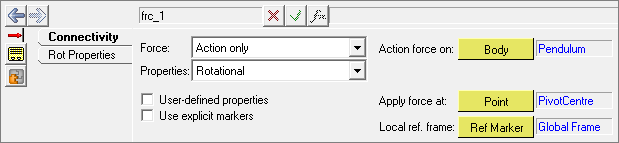
-
On the Connectivity tab, add a second force, frc_1,
label it PivotTorque, and set the Connectivity properties
as follows:
Modifying the MBS Model for Co-Simulation
Modify the basic MBS model for co-simulation by adding MotionView entities including solver arrays and solver variables.
Adding Solver Variables
-
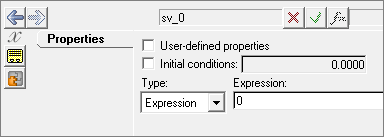
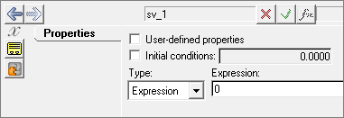
Create two solver variables: ControlForce (varname: sv_0)
and PivotTorque (varname: sv_1) as follows:
-
Connect the two solver variables to the forces you created in the previous
section, Adding Forces.
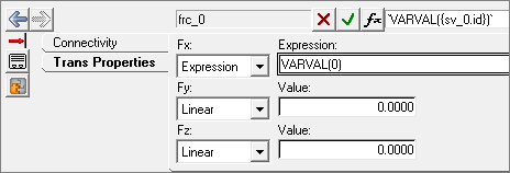
As you see in the following figure, on the Trans Properties tab for ControlForce, for Fx, select Expression, and for f, enter: `VARVAL({sv_0.id})`. This expression specifies the ControlForce to be the first solver variable, sv_0. This variable sets the control signal sent from Activate to be the control force acting on the translational joint of the Cart.
-
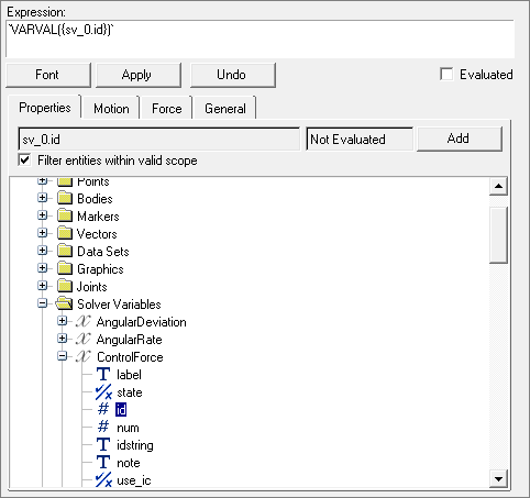
Verify that the varnames match (sv_0): From the Expression
Builder, select the solver variable by name and enter its ID as you see in the
following figure:
-
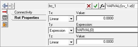
On the Rot Properties tab for PivotTorque, for Ty, select
Expression, and then for f,
enter:`VARVAL({sv_1.id})`. This expression sets the
PivotTorque as the second solver variable, sv_1, which
specifies the control signal sent from Activate as
the torque acting on the rotation of the pendulum.
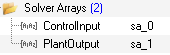
-
Insert two solver arrays. Label them ControlInput and
PlantOutput.
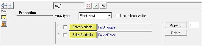
-
The ControlInput solver array includes both the PivotTorque and ControlForce
solver variables. Set the properties as follows:
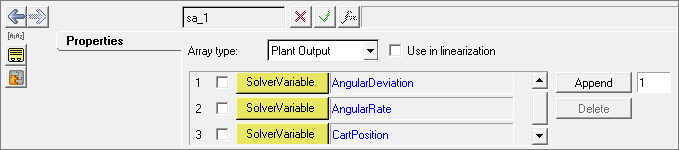
-
The PlantOutput solver array includes the following solver variables:
AngularDeviation, AngularRate and CartPosition. Set the Plant Output properties
as follows:
-
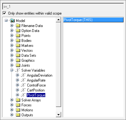
To help you select the proper solver variable names, click
 and a panel appears:
Validating the Inverted Pendulum Model
Simulate the MBS model in MotionSolve and validate that it performs as required.
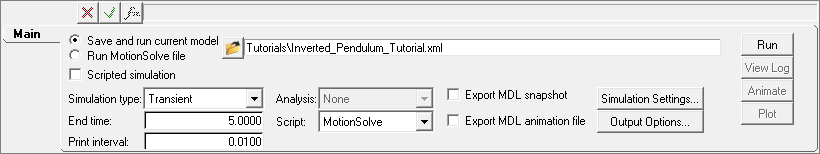
-
From the Run panel, save your model as an XML file. This file is used for the
solver run as well as the Activate model. Alternatively, you can run the
MotionView .mdl file, and name it
Inverted_Pendulum_Tutorial.xml.
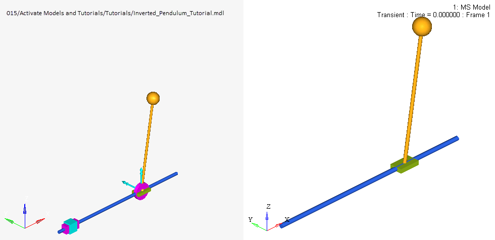
-
Animate the results from the simulation and confirm that the model works as
intended before continuing to the next steps. The controller is not yet
connected to the model, therefore the input force and torque are zero.
Building the Controls System Model
Build a controls system model with Activate.
The controls system model requires these blocks:
| Block | Description |
|---|---|
| MotionSolve | Enables the embedding of a MotionSolve model into an Activate model. |
| Mux | Reads multiple signals into one signal. |
| Demux | Reads a signal which contains multiple components and splits the signal into individual components. |
| OMLCustomBlock | |
| Scope | Plots data as defined. |
| Constant | Generates a command signal. |
| PID | Serves as the controller block, the brain of the model. |
| Sum | Calculates the error from reference signals and feedback. |
Creating the Diagram of the Activate Model
-
On the block, PID1_AngularDeviation, double-click, and
enter these values for the parameters:
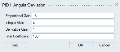 Note:
Note:- Proportional Gain multiplies the error signal by a constant gain Kp.
- Integral Gain multiplies the sum history of error with integral gain Ki.
- Derivative Gain multiplies the rate of change of error with gain Kd.
-
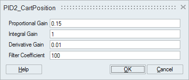
On the block, PID2_CartPosition, double-click. In the
dialog, define the parameters:
-
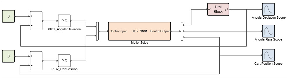
All of the required blocks are now present. Assemble and link the blocks in the
diagram as follows:
Simulating the Diagram
-
On the ribbon, select Setup.

-
On the ribbon, select Run.

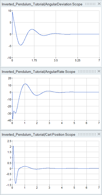
The Scope blocks in the model generate the following plots for the cart: Angular Deviation, Angular Rate and Cart Position.