Computation of iron losses: about
Introduction
Magnetic losses (or iron losses) computation is a subsequent computation, carried out in Flux post-processor.
This chapter introduces iron losses computation, from modified Bertotti formulas, or with LS model (Loss Surface).
- the magnetic losses in the magnetic circuits (also called ‘iron losses’)
- the losses by Joule effect in coils (also called ‘copper losses’)
- the mechanical losses (mainly by friction in rotating machines)
Losses in magnetic materials:
- The hysteresis losses (microscopic Eddy currents) are associated to currents at a small scale. These currents are the result of local induction variation caused by the magnetic structure in movement (essentially wall movement).
- The Foucault losses (macroscopic Eddy current), are due to the excitation frequency. They appear when domain wall displacement increases due to frequency increase.
Magnetic losses and hysteresis cycle:
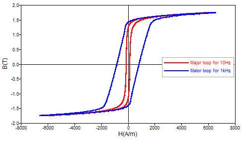
- the volume energy created by hysteresis losses is corresponding to static hysteresis cycle (f<1Hz).
- as the frequency increases, the cycle area increases and the volume energy created by eddy current losses is corresponding to the difference between the dynamic hysteresis cycle area and the static one.

Figure 1. Major cycles for different frequencies
Access to computation of iron losses
- For modified Bertotti model: Steady state AC magnetic (averaged iron losses computation) and transient magnetic (averaged or instantaneous iron losses computation)
- For LS model: Transient magnetic only (averaged or instantaneous iron losses computation)
Computation of iron losses
The computation box of iron losses can be accessed in the post-processing context via
Computation type
- On regions : enables to compute modified Bertotti or LS iron losses on a selection of laminated regions. The iron losses model can be defined on the material or in this box via Model for losses field. The computation gives instant losses and averaged losses on the time interval for a set of fixed geometric parameters or fixed I/O parameters.
- Multi-parametric on regions : enables to compute modified Bertotti or LS iron losses on a selection of laminated regions. The iron losses model can be defined on the material or in this box via Model for losses field. The computation gives instantaneous losses for several sets of geometric parameters or I/O parameters. This computation can be used in optimizations or efficiency maps.
- On point with LS model defined in the material: this option can only be accessed in transient magnetic application. This calculus enables to compute LS iron loss volume densities on a point in a laminated region. Iron losses model must be defined in the material or the user can also load his own losses file, see : LS model identification with MILS. The computation gives instantaneous losses and averaged losses volume densities on the time period for a set of fixed geometric parameters or I/O parameters. With this computation, it is possible to display the hysteresis cycle.