Shape Optimization
Introduction
In Flux, a shape optimization may be run in Magneto-Static or in Transient Magnetic applications of the Flux 2D module in Beta mode only on Windows, to do this the user must define an optimization problem. An optimization problem defines the objective function and the constraints as seen in this part.
- Adjoint method
- Coupling with Optistruct
- How to set up a Shape optimization in Flux
- Limitations
- Example of application
Adjoint method
Based on the movement of the mesh nodes and not on geometrical entities such as lines, the adjoint method allows the computation of a semi-analytical sensitivity with a reduced computation time compared to finite difference. While keeping the regions and materials bounds and prevents overlapping of mesh elements, the mesh nodes will move into the most attractive direction defined by the sensitivity computation on the objective function over a computation scenario. In Flux this method requires structural informations such as the lines to move of the electromagnetic design, it also requires to define an optimization problem (response, objective function, constraints) and to define a solving scenario. It must be keeped in mind that only the mesh is moving and not the geometrical entities, however with the macro named CreateGeomFromOS.PFM in the folder .../Extensions/Macros/Macros_Flux2D_Shape_Optimization, it is possible to rebuild geometrical entities such as lines and points from the mesh nodes. For more informations dealing with the adjoint method, see this page.
Coupling with Optistruct
- Install OptiStruct 2021.1 available on https://altairone.com/Marketplace
- Set the OptiStruct installation path in the Flux Supervisor > Options > Coupled software and add your local installation path such as: C:\Program files\Altair_2021\hwsolvers\scripts
How to set up Shape Optimization in Flux
- In the data tree on the left, in the Solver, then in the Optimization node, select the node Responses, choose a response in the short list, a response is a physical quantity that will take part of the optimization problem, the list of each available response is summarized here, the responses are the physical quantity to be optimized.
- Select now the node Constraints in the data tree. Three types of constraints may be defined: a structural constraint with its lower and upper bounds for volume constraints, a constraint on node displacement may be setted with the axis or double axis symmetry constraint and a constraint on physical quantities using one or several Responses. For more information about these constraints, see this page. It is not mandatory to have a constraint in the optimization problem to run a shape optimization in Flux;
- Select the node Optimization problem:
- Set the field Minimization or maximization on the chosen value, this field allows the user to choose if the objective function must be increased or decreased.
- In the field Objective function to optimize, set the operation to apply on the objective function, it can be defined on the available short list, or with a custom function defined with Compose, if the function is defined with Compose, an additional parameter will be required such as the function's name. An oml file type may be used to defined an objective function and several constraints.
- Select the Responses and the Constraints previously
definedNote: Several responses may be selected at the same time, in Flux this feature is named Multi-response where a linkage is operated between all the values. Be sure that all the responses are in the same range of values.Note: Several constraints may be selected also at the same time.
- In the Solving menu, choose Run Shape Optimization, it asks
you to:
- Select the lines where the nodes of the mesh can move
- Choose a solving scenario
- Select a working directory for the temporary files created during the optimization
- Choose your optimization problem previously defined
- To set different options on the optimizer, see the node Optimization options, more informations are available on this page
Limitations
- No remeshing during the solving scenario (including the variation of geometrical parameters, compressible mechanical sets)
- No adaptative time step during solving
- Some restrictions about the selected lines (no lines at the interface between two faces with the same material on both sides, no lines on the sliding cylinder)
- The mesh in the zone to optimize must be thin and regular
Example
This example may be seen as an extension of the example available in the supervisor in the 2D Application Note section named: Shape Optimization of a synchronous reluctance machine
Let's consider the modeling of the following electrical machine represented by only one quarter of the full device.
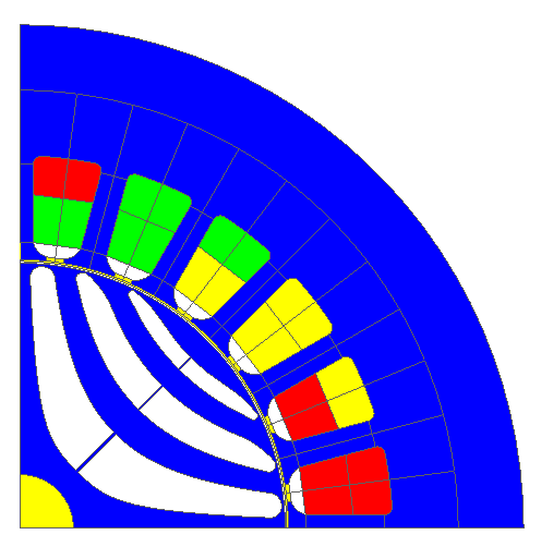
Figure 1. Four poles electrical machine with three current phasis
- Reduce the weight of the rotor
- Increase the mean value of the torque
To run the shape optimization, the selected response is the Torque as explained in this page, a path to compute the torque is depicted in the following figure:
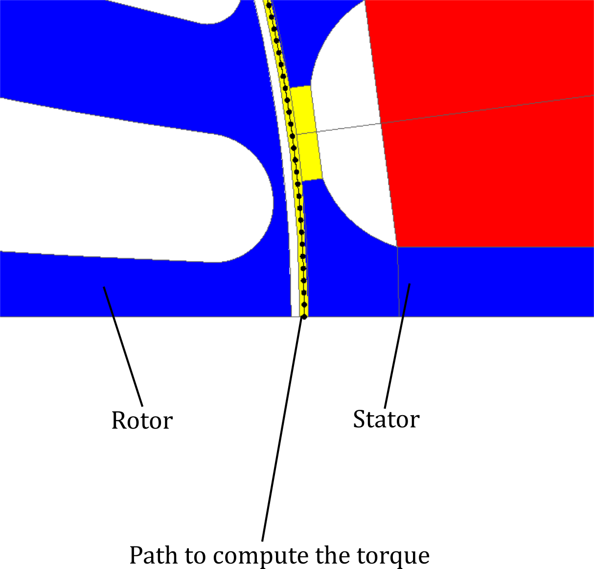
Figure 2. Description of the path to compute the torque with Maxwell's tensor approach
- A one axis symmetry constraint
- A constraint on the volume of the rotor in order to decrease its weight
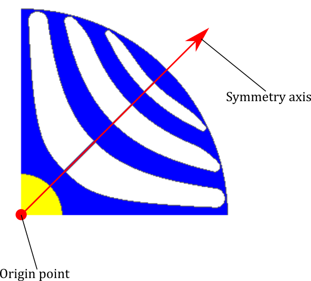
Figure 3. Origin point and symmetry axis for the one axis symmetry constraint
The origin axis is setted to (0,0) and the symmetry axis is setted to (0.5,0.5).
For the constraint on the volume, we want to reduce the volume of iron in the rotor about 20%, in the upper bound the value corresponding to 80% of the total volume is filled, in the lower bound 60% of the volume is filled.
Even if at the starting point the initial design is not between the bounds, the optimization algorithm will deteriorate the objective function in order to find a design that fit the bounds, then the algorithm will start to optimize the design in order to increase or decrease the objective function.
In the objective function, we choose to Maximize the Average of the Torque response previously defined
In the end, the lines where the nodes can move are selected as depicted in the figure bellow (the lines are surrounded in yellow):
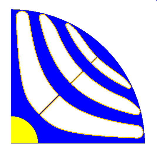
Figure 4. Lines to be considered during the optimization process
The scenario is piloted by the mechanical set angle and is covering an electrical period with two degrees per computation step.
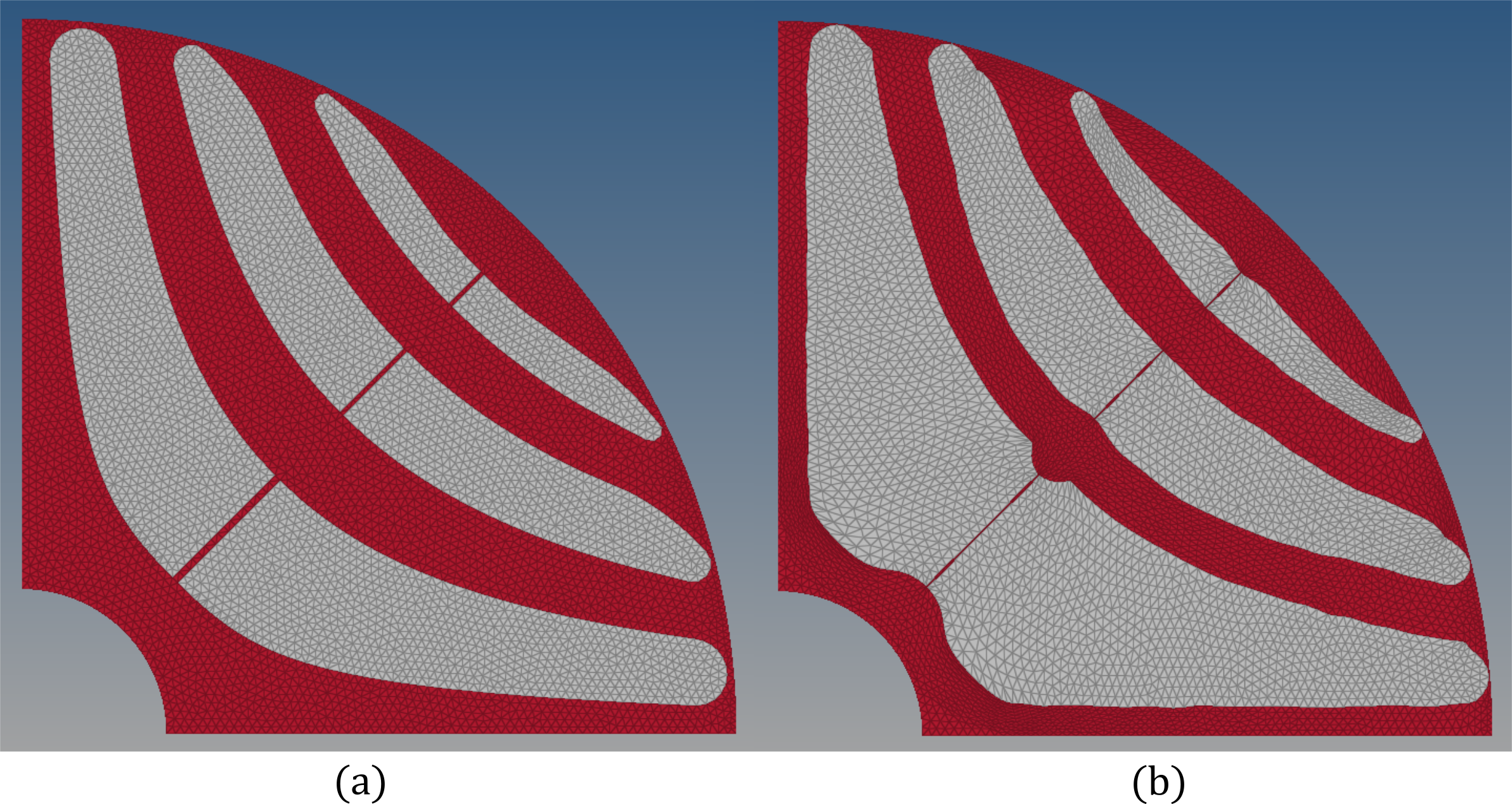
Figure 5. Initial design of the reluctance synchronous machine (a) and final design of the reluctance synchronous machine (b)
| Initial design | Final design | Difference | |
|---|---|---|---|
| Mean torque (N.m) | 11.9 | 12.5 | + 4.8% |
| Rotor weight (kg) | 0.5 | 0.4 | - 20% |
Figure 6. Displacement of the nodes during the optimization process