ACU-T: 3100 Conjugate Heat Transfer in a Mixing Elbow
Prerequisites
Prior to starting this tutorial, you should have already run through the introductory HyperWorks tutorial, ACU-T: 1000 HyperWorks UI Introduction, and have a basic understanding of HyperWorks CFD and AcuSolve. Although it is not necessary, it is recommended that you complete ACU-T: 2000 Turbulent Flow in a Mixing Elbow prior to running this simulation. To run this simulation, you will need access to a licensed version of HyperWorks CFD and AcuSolve.
Prior to running through this tutorial, click here to download the tutorial models. Extract ACU-T3100_MixingElbowHeatTransfer.hm from HyperWorksCFD_tutorial_inputs.zip.
Problem Description
The problem to be addressed in this tutorial is shown schematically in Figure 1. It consists of a mixing elbow made of stainless steel with water entering through two inlets with different velocities and at different temperatures. The geometry is symmetric about the XY midplane of the pipe, as shown in the figure.

Figure 1. Schematic of Mixing Elbow with Stainless-steel Walls
Start HyperWorks CFD and Open the HyperMesh Database
-
From the Home tools, Files tool group, click the Open Model tool.

Figure 2.The Open File dialog opens.
Validate the Geometry
The Validate tool scans through the entire model, performs checks on the surfaces and solids, and flags any defects in the geometry, such as free edges, closed shells, intersections, duplicates, and slivers.
Figure 3.
Set Up the Problem
Set Up the Simulation Parameters and Solver Settings
-
From the Flow ribbon, click the Physics tool.

Figure 4.The Setup dialog opens. -
Under the Physics models setting:
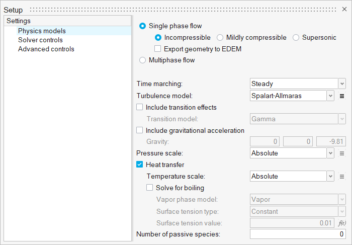
Figure 5. -
Click the Solver controls setting and verify that the
parameters are set as shown in the figure below.
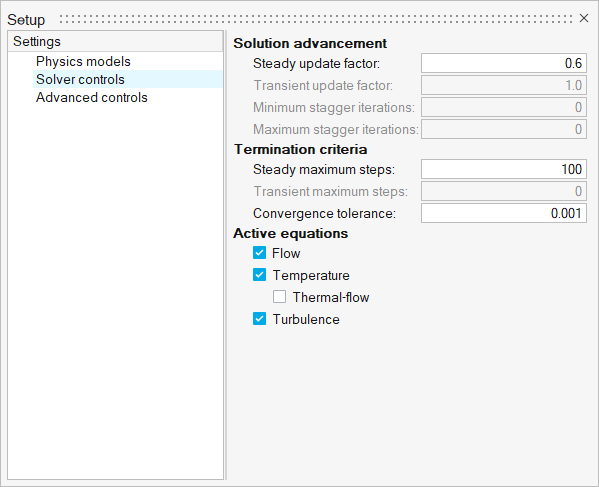
Figure 6.
Create a New Material Model
-
From the Flow ribbon, click the Material Library tool.

Figure 7.The Material Library opens. -
Click the My Materials tab then click
 to
create a new solid.
A material creation dialog opens.
to
create a new solid.
A material creation dialog opens. -
Change the Density value to 8030.
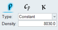
Figure 8. -
Change the Specific heat value to 500.
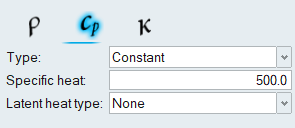
Figure 9. -
Change the Conductivity value to 16.2.
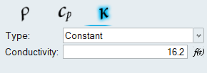
Figure 10. -
Exit the material creation dialog.
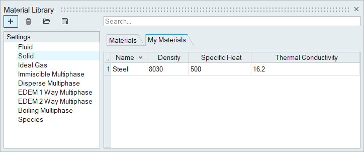
Figure 11.
Assign Material Properties
-
From the Flow ribbon, click the Material tool.

Figure 12. -
Select the outer pipe solid.
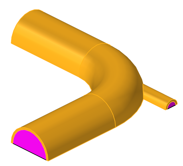
Figure 13. -
On the guide bar, click
 to execute the command and remain in the
tool.
to execute the command and remain in the
tool.
-
Next, select the inner pipe solid.
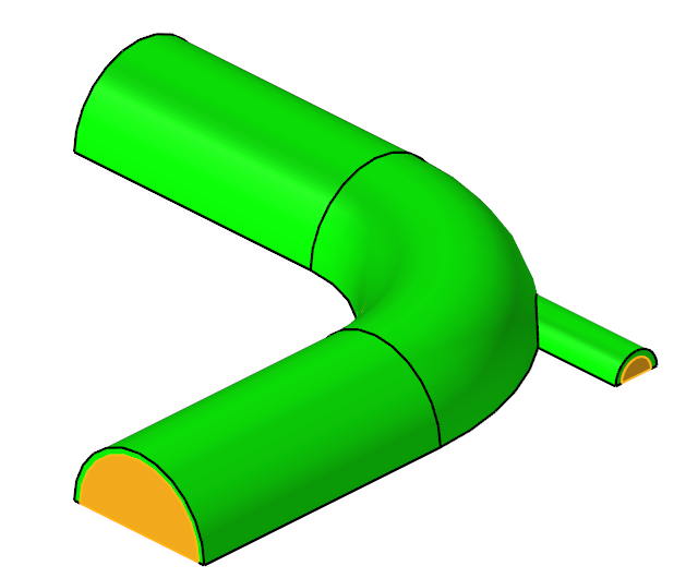
Figure 14. -
On the guide bar, click
 to execute
the command and exit the tool.
to execute
the command and exit the tool.
Assign Flow and Thermal Boundary Conditions
Set Boundary Conditions for the Large Inlet
-
From the Flow ribbon, Profiled
tool group, click the Profiled Inlet tool.

Figure 15. -
Click the face of the large inlet.
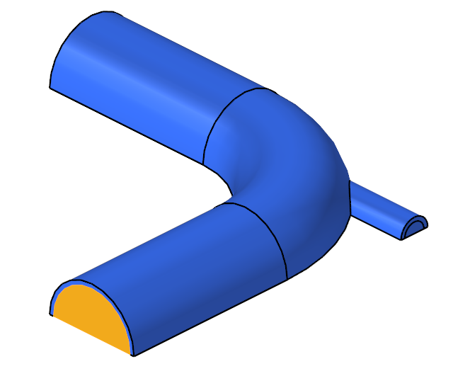
Figure 16. -
On the guide bar, click
to execute the command and remain in the
tool.
Note: The number of inlets created appears in parenthesis on the top-right of the Profiled tool icon.
Set Boundary Conditions for the Small Inlet
-
Click the face of the small inlet.
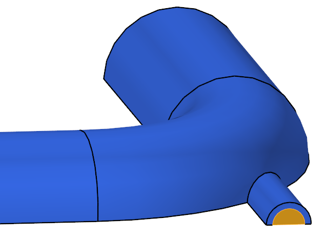
Figure 17. -
On the guide bar, click
to execute
the command and exit the tool.
Set Boundary Conditions for the Outlet
-
From the Flow ribbon, click the Outlet tool.

Figure 18. -
Click the face of the outlet.
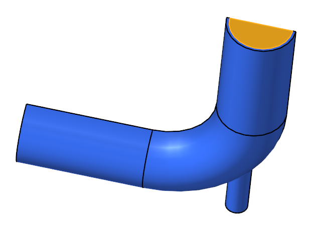
Figure 19. -
In the microdialog, make sure both
Static pressure and Pressure loss factor are 0.
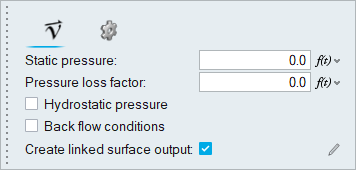
Figure 20. -
On the guide bar, click
to execute
the command and exit the tool.
Set Boundary Conditions for the Symmetry Planes
This geometry is symmetric about the XY midplane, and can therefore be modeled with half of the geometry. In order to take advantage of this, the midplane needs to be identified as a symmetry plane. The symmetry boundary condition enforces constraints such that the flow field from one side of the plane is a mirror image of that on the other side.
-
From the Flow ribbon, click the Symmetry tool.

Figure 21. -
Click the face of the symmetry plane.
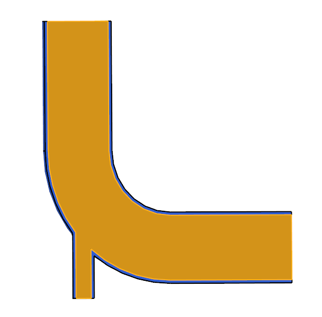
Figure 22. -
In the microdialog, accept the
default symmetry conditions.
Figure 23. -
On the guide bar, click
to execute the command and remain in the
tool.
-
Next, select the faces for the pipe wall symmetry.
Figure 24. -
On the guide bar, click
to execute
the command and exit the tool.
Set Boundary Conditions for the Outer Pipe Walls
-
From the Flow ribbon, click the No Slip tool.

Figure 25. -
Click the faces of the outer pipe walls.
Figure 26. -
In the microdialog, click
 to open
the temperature tab.
to open
the temperature tab.
-
Change the Convective heat resistance temperature value to
302.594.
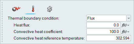
Figure 27. -
On the guide bar, click
to execute
the command and exit the tool.
Generate the Mesh
-
From the Mesh ribbon, click the
Volume tool.

Figure 28.The Meshing Operations dialog opens.Note: If the model has not been validated, you are prompted to create the simulation model before running the batch mesh. -
Accept all other default parameters.
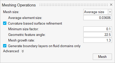
Figure 29. -
Observe the refined mesh around the pipe walls.
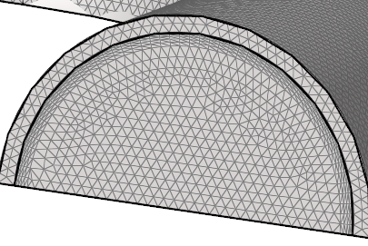
Figure 30.
Run AcuSolve
-
From the Solution ribbon, click the Run tool.

Figure 31.The Launch AcuSolve dialog opens. -
Leave the remaining options as default and click
Run to launch AcuSolve.
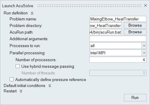
Figure 32.The Run Status dialog opens. Once the run is complete, the status is updated and you can close the dialog.Tip: While AcuSolve is running, right-click on the AcuSolve job in the Run Status dialog and select View Log File to monitor the solution process.
Post-Process the Results with HW-CFD Post
-
Click
 and set the Colormap Name to Rainbow
Uniform.
and set the Colormap Name to Rainbow
Uniform.
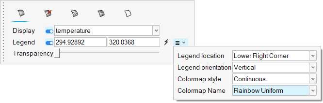
Figure 33. -
Click
 on the guide bar.
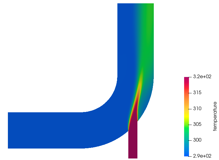
Figure 34. -
Click the Right face on the View Cube to align the
model.
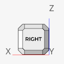
Figure 35.Tip: If the orientation is not the standard, click the face again to re-align the model back to the standard orientation. -
Click
 to reset the range.
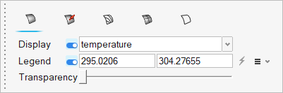
Figure 36. -
Click on the guide bar.
Figure 37.
Summary
In this tutorial, you learned how to set up a conjugate heat transfer simulation using HyperWorks CFD and how to create a new material model. You launched AcuSolve directly from HyperWorks CFD to compute the solution and then post-processed the results using the Post ribbon.