ACU-T: 5000 Centrifugal Air Blower with Moving Reference Frame (Steady)
Prerequisites
Prior to starting this tutorial, you should have already run through the introductory tutorial, ACU-T: 1000 Basic Flow Set Up, and have a basic understanding of HyperWorks CFD and AcuSolve. To run this simulation, you will need access to a licensed version of HyperWorks CFD and AcuSolve.
Prior to running through this tutorial, click here to download the tutorial models. Extract ACU-T5000_BlowerSteady.hm from HyperWorksCFD_tutorial_inputs.zip.
Problem Description
The problem to be addressed in this tutorial is shown schematically in Figure 1 and Figure 2. It consists of a centrifugal blower with a wheel of forward curved blades, and a housing with inlet and outlet ducts. The fluid through the inlet plane enters the hub of the blade wheel, radially accelerates due to centrifugal force as it flows over the blades, and then exits the blower housing through the outlet plane. Because they're relatively cheaper and simpler than axial fans, centrifugal blowers have been widely used in HVAC (heating, ventilating, and air conditioning) systems of buildings.

Figure 1. Schematic of Centrifugal Blower
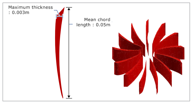
Figure 2. Schematic of Fan Blades
The boundary condition at the inlet is taken as stagnation pressure rather than mass flow rate so that AcuSolve calculates pressure rise based on impeller rotation.
The fluid in this problem is air, which has a density (ρ) of 1.225 kg/m3 and a viscosity (μ) of 1.781 x 10⁻⁵ kg/m-sec.
Start HyperWorks CFD and Open the HyperMesh Database
-
From the Home tools, Files tool group, click the Open Model tool.

Figure 3.The Open File dialog opens.
Validate the Geometry
The Validate tool scans through the entire model, performs checks on the surfaces and solids, and flags any defects in the geometry, such as free edges, closed shells, intersections, duplicates, and slivers.
Figure 4.
Set Up the Problem
Set Up the Simulation Parameters and Solver Settings
-
From the Flow ribbon, click the Physics tool.

Figure 5.The Setup dialog opens. -
Under the Physics models setting:
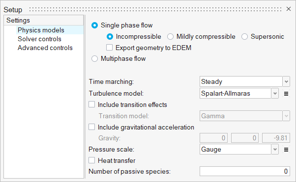
Figure 6. -
Click the Solver controls setting and verify that the
parameters are set as shown in the figure below.
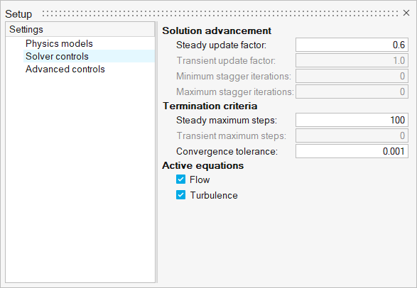
Figure 7.
Assign Material Properties
-
From the Flow ribbon, click the Material tool.

Figure 8. -
Using window selection, draw a box around the entire model.
Both the centrifugal blower and the housing solids are selected.
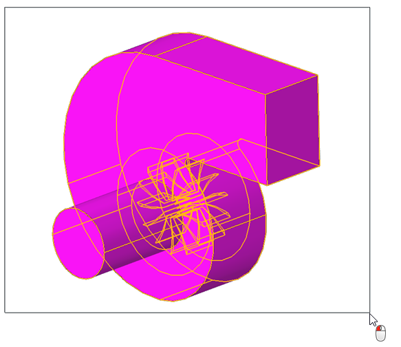
Figure 9. -
On the guide bar, click
 to execute
the command and exit the tool.
to execute
the command and exit the tool.
Define the Reference Frame
In this step, you will create a rotating reference frame for the fluid in the impeller region so that the elements in those regions are solved in the given rotating reference frame and rotational body forces are added to that volume set.
-
Hide the housing solid.
- Set the entity selector to Solids.
- Select the centrifugal housing.
- Right-click and select Hide form the context menu or press H.
Only the solid for the centrifugal blower displays in the modeling window.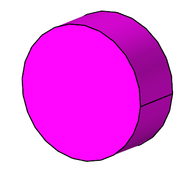
Figure 10. -
From the Flow ribbon, click the Reference Frame tool.

Figure 11. -
Define the axis of rotation.
-
Use the Surf Center snap point to place the axis in the middle of the
centrifugal blower.
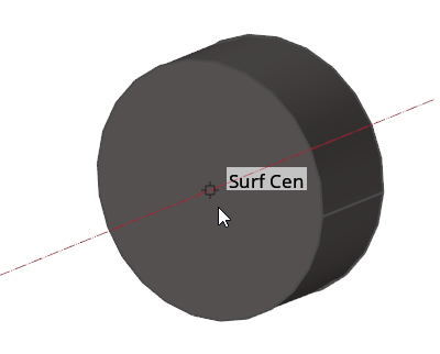
Figure 12. -
Click
 to flip the spin direction.
-
Enter a value of 157.09 in the text field.
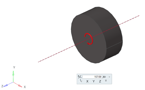
Figure 13.
-
Use the Surf Center snap point to place the axis in the middle of the
centrifugal blower.
-
On the guide bar, click
to execute
the command and exit the tool.
Define Flow Boundary Conditions
-
From the Flow ribbon, Pressure
tool group, click the Stagnation Pressure tool.

Figure 14. -
Click the face of the inlet.
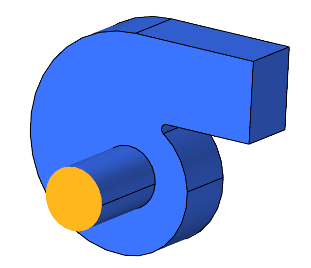
Figure 15. -
Set the Turbulence viscosity ratio to 10.
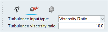
Figure 16. -
On the guide bar, click
to execute
the command and exit the tool.
-
Click the Outlet tool.

Figure 17. -
Click the face of the outlet.
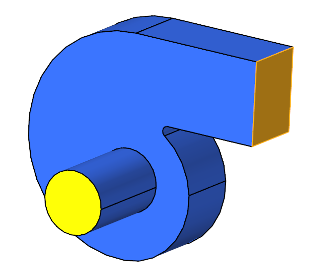
Figure 18. -
In the microdialog, make sure both Static pressure and Pressure loss
factor are 0.
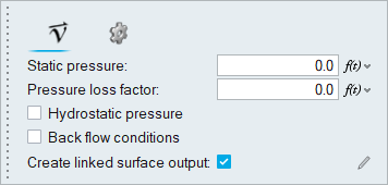
Figure 19. -
On the guide bar, click
to execute
the command and exit the tool.
Generate the Mesh
-
From the Mesh ribbon, click the
Volume tool.

Figure 20.The Meshing Operations dialog opens.Note: If the model has not been validated, you are prompted to create the simulation model before running the batch mesh. -
Accept all other default parameters.
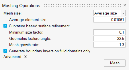
Figure 21.
Define a Surface Monitor and Run AcuSolve
-
Right-click and select Hide form the context menu or
press H.
The solid for the centrifugal blower should be displayed in the modeling window
Figure 22. -
From the Solution ribbon, click the Surfaces tool.

Figure 23. -
Select the blower interface and verify that the arrow is heading toward the
blower, as shown in figure below.
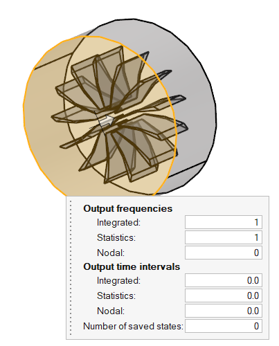
Figure 24. -
On the guide bar, click
to execute
the command and exit the tool.
-
From the Solution ribbon, click the Run tool.

Figure 25.The Launch AcuSolve dialog opens. -
Leave the remaining options as default and click
Run to launch AcuSolve.
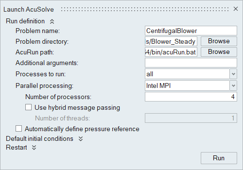
Figure 26.Tip: While AcuSolve is running, right-click on the AcuSolve job in the Run Status dialog and select View Log File to monitor the solution process.
Plot Ratios and Surface Output
-
In the Plot Utility dialog, double-click on
Residual Ratio to open the corresponding plot.
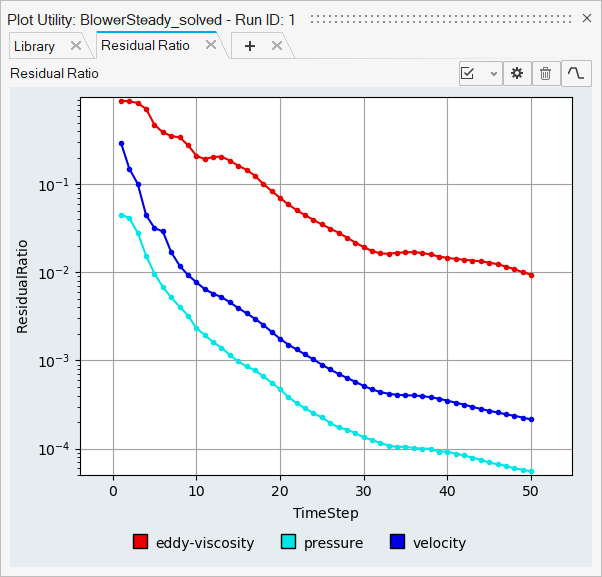
Figure 27.The plot shows the residuals of the equations as the solution progresses through each time step.
You can see the residuals dropping smoothly. Once the pressure and velocity residual ratios reach a value less than the specified convergence tolerance (0.001), the solution is considered to be converged.
By default, the eddy viscosity convergence tolerance is set to a magnitude of one order higher than the specified convergence tolerance (0.01).
-
Click the Logarithm icon
 to change the solution ratio into a log scale.
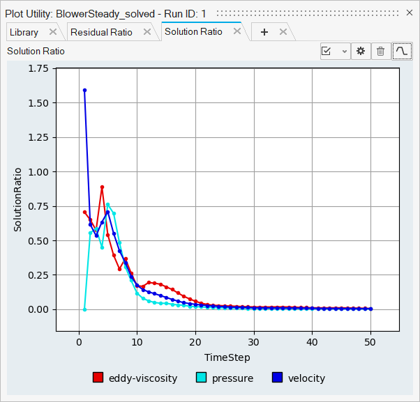
Figure 28.The plot shows the solution convergence.
Once the pressure and velocity residual ratios reach a value less than the specified convergence tolerance (0.01), the solution is considered to be converged.
By default, the eddy viscosity convergence tolerance is set to a magnitude of one order higher than the specified convergence tolerance (0.1).
-
Click
 to add a new plot.
-
Under the Y-Axis heading, click the arrow besides Run
Data and select Surface Output
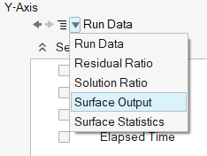
Figure 29. -
Select blades for the surface output.
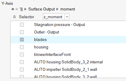
Figure 30. -
Click Create.
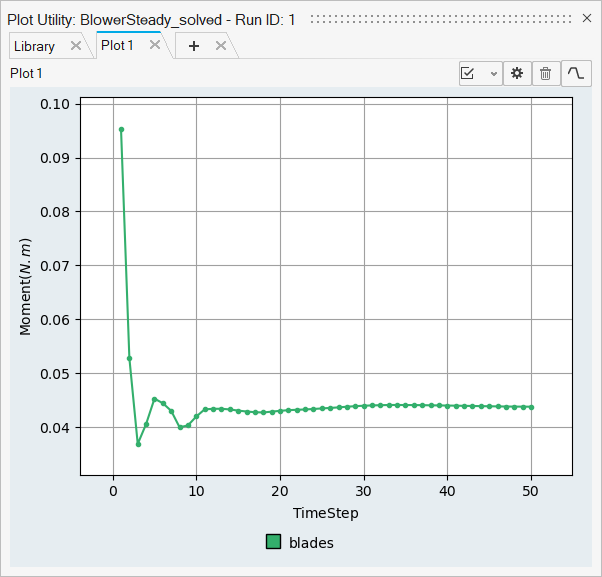
Figure 31. -
Click to add a new plot.
-
Click Create.
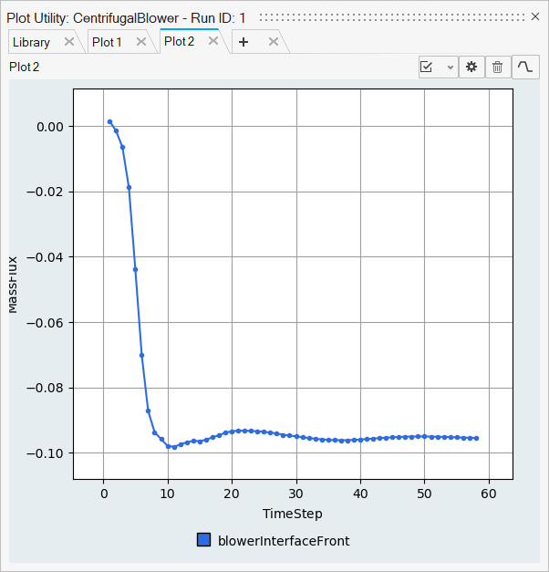
Figure 32.
Post-Process the Results with HW-CFD Post
Plot Pressure on a Slice Plane
-
Click the Slice Planes tool.

Figure 33. -
In the microdialog, click
 and move the plane along its normal direction a distance of
-0.07.
and move the plane along its normal direction a distance of
-0.07.
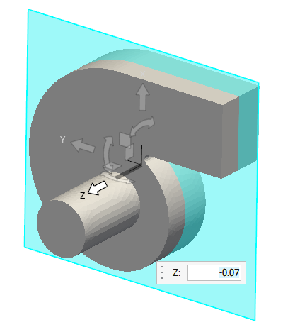
Figure 34. -
In the slice plane microdialog, click
 to
create the slice plane.
to
create the slice plane.
-
Click
 and set the Colormap Name to Rainbow
Uniform.
and set the Colormap Name to Rainbow
Uniform.
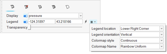
Figure 35. -
On the guide bar, click
to execute
the command and exit the tool.
-
In the Post Browser, hide all the Parts and Flow
Boundaries.
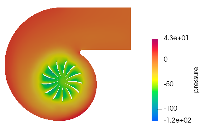
Figure 36.
Plot Velocity Streamlines
-
Click the tool.

Figure 37. -
In the microdialog, click
and move the plane along its normal direction a distance of
-0.07.
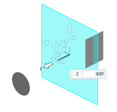
Figure 38. -
In the slice plane microdialog, click
 and set the circle radius to 0.1.
-
Click Calculate.
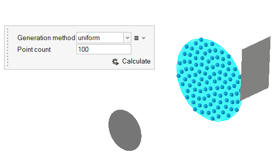
Figure 39. -
On the guide bar, click
to execute
the command and exit the tool.
-
Click
 on the guide bar.
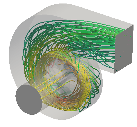
Figure 40.
Summary
In this tutorial, you successfully learned how to set up a steady state simulation involving a rotating reference frame in a centrifugal blower. You started by importing the mesh and then once the case was set up, you generated a solution using AcuSolve. Then, you computed the blower momentum using the Plot Utility and created a contour plot for pressure and velocity streamlines using HyperWorks CFD post.