ACU-T: 5403 Piezoelectric Flow Energy Harvester: A Fluid-Structure Interaction
This tutorial provides the instructions for setting up, solving and viewing results for a simulation of a piezoelectric fluid harvester. In this simulation, a piezoelectric flow harvester is placed in a fluid flow channel. The harvester is attached to a cylinder mount which also acts as a bluff body causing vortices in the fluid flow. The interaction between the pressure fields generated by the vortices and the flow harvester structure is simulated in this tutorial. HyperWorks CFD is used in conjunction with a structural solver to compute the structural displacement of the harvester using a direct-coupled fluid structure interaction (DC-FSI) approach. Arbitrary Lagrangian Eulerian (ALE) approach is used to compute the mesh deformation in the fluid domain as it interacts with the deforming structure.
- Set up a Direct Coupled FSI simulation (DC-FSI)
- HyperWorks CFD/OptiStruct multiphysics coupling
- Setting up external code parameters to support coupling
- Assigning external code parameters to surfaces
- Analyze the problem
- Start HyperWorks CFD and create a simulation database
- Import the mesh for the simulation.
- Set general problem parameters
- Set the appropriate boundary conditions for the coupling surfaces
- Run OptiStruct
- Run HyperWorks CFD
- Monitor the solution with HyperWorks CFD
- Post-process the nodal output with HyperWorks CFD
- Create an animation for the transient simulation with HyperWorks CFD Post
Prerequisites
You should have already run through the introductory tutorial, ACU-T: 2000 Turbulent Flow in a Mixing Elbow. It is assumed that you have some familiarity with HyperWorks CFD and AcuSolve. You will also need access to a licensed version of AcuSolve.
The coupled structural solver used for this tutorial is another HyperWorks product, OptiStruct. Thus, to follow this tutorial you will also need access to a licensed version of OptiStruct. The corresponding OptiStruct setup for this tutorial is available in the OptiStruct tutorial manual.
Prior to running through this tutorial, click here to download the tutorial models. Extract ACU-T5403_Harvester_DCFSI.hm and slab_dcfsi.fem from HyperWorksCFD_tutorial_inputs.zip. The file ACU-T5403_Harvester_DCFSI.hm stores the geometry information for the fluid portion of the model for this problem, and the file slab_dcfsi.fem is the OptiStruct input deck for this problem.
The color of objects shown in the modeling window in this tutorial and those displayed on your screen may differ. The default color scheme in HyperWorks CFD is "random," in which colors are randomly assigned to groups as they are created. In addition, this tutorial was developed on Windows. If you are running this tutorial on a different operating system, you may notice a slight difference between the images displayed on your screen and the images shown in the tutorial.
Analyze the Problem
An important step in any CFD simulation is to examine the engineering problem at hand and determine the important parameters that need to be provided to HyperWorks CFD. Parameters can be based on geometrical elements (such as inlets, outlets, or walls) and on flow conditions (such as fluid properties, velocity).
The schematics of the problem is shown in Figure 1. The CFD model consists of a cylindrical body and a cantilever beam. This cylindrical body generates vortex shedding. This vortex shedding creates a zone of alternating asymmetric pressure distribution on either side of the beam. Such an alternating pressure distribution exerts an oscillating force on the beam, creating a sustainable oscillating vibration in the beam.
The fluid solver does not require the solid body to be modeled. However, the structural solver will solve for the structural deformation using the fluid flow and pressure field which will be acting on the surface of the structure. The information required by the structural solver for structure displacement calculation will be passed on to it by the fluid solver. The structural solver on the other hand, will pass on the displacement information to the fluid solver. The fluid solver will then use this displacement information to calculate the flow field at the next time step, which will then be used by the structural solver to update the displacement information. This back and forth exchange of information between the fluid and structural solver will take place at each time step, and continue until one of the solvers signals the end of simulation. Figure 2 shows the arrangement of the beam with its various layers.

Figure 1. Schematic of the Problem

Figure 2. The Beam with its Various Layers
Fluid Structure Interaction
Fluid Structure Interaction is the interaction between a fluid flow and a deformable solid structure in contact with this flow. An FSI problem can be an external or an internal flow problem. The fluid flow can be external with the solid body immersed in the flow, for example, a windmill blade in open atmosphere. The fluid flow can also be internal with the solid body enclosing the flow, for example, fluid flow inside a deformable pipe. In both cases, the principle behind solving the problem remains the same. When a fluid flow encounters a structure, fluid pressure exerts a stress on the solid body that can lead to deformations in the structure. The magnitude of the deformation depends on the stiffness of the structure material and the magnitude of pressure force exerted by the fluid. The deformation in the structure shape then leads to altering of the flow characteristics in vicinity of the structure.
- Practical-FSI (P-FSI): The structure is reduced in the modal space and coupled to the fluid domain through interface nodes. The coupling between the solvers happens in a single pass itself. Structural behaviour is limited to be linear in a P-FSI simulation.
- Direct coupling (DC-FSI): The coupling is a co-simulation between the structural and the fluid solver, with each solver stepping through time simultaneously and iterating to equilibrium in each time step.
In case the deformations in the structure are large enough to alter the fluid flow significantly, the DC-FSI co-simulation approach should be used. With this approach, as the fluid flow and pressure fields affect the structural deformations, and the structural deformations affect the flow and pressure, the information about these effects is exchanged between the solvers in real time.
Given the difference in coupling methodology, it is likely that slightly different results will be observed when a same problem is solved using P-FSI and DC-FSI approaches. The choice of the approach that should be used shall depend on the problem and the available resources. As mentioned above, the P-FSI approach should be limited to the cases when displacements in the structure are small, and the structural behaviour can be approximated to be linear. For all other cases, DC-FSI should be preferred. However, DC-FSI simulations incur a higher computational resources cost. With this consideration, P-FSI simulation can also be used as a preliminary test simulation before a DC-FSI simulation is carried out.
FSI can be stable or oscillatory. In a stable FSI, the deformed shape of the structure will not change with time, unless the flow changes as well. In an oscillatory FSI, once the structure is deformed, it will try to return to its non-deformed state and then the whole deformation process repeats itself.
Mesh Motion Approaches in HyperWorks CFD
- Arbitrary Lagrangian Eulerian (ALE)
- Interpolated Mesh Motion.
Arbitrary Lagrangian Eulerian (ALE)
ALE is an approach for mesh motion in which the computational nodes are moved arbitrarily with the aim of optimizing the element quality. An additional Partial Differential Equation (PDE) is solved to arrive at the appropriate mesh position. ALE is capable of handling complex arbitrary motions and is therefore the most general approach in simulating moving mesh problems. Generality comes with additional computational cost because of the extra PDE to be solved. For simpler motions like 1D or 2D motions faster approaches are available which include interpolated mesh motion, general specified motions, nodal boundary conditions based approaches.
Start HyperWorks CFD and Open the HyperMesh Database
-
From the Home tools, Files tool group, click the Open Model tool.

Figure 3.The Open File dialog opens.
Validate the Geometry
The Validate tool scans through the entire model, performs checks on the surfaces and solids, and flags any defects in the geometry, such as free edges, closed shells, intersections, duplicates, and slivers.
Figure 4.
Set Up Flow
Set Up the Simulation Parameters and Solver Settings
-
From the Flow ribbon, click the Physics tool.

Figure 5.The Setup dialog opens. -
Under the Physics models setting:
- Verify that the Incompressible option is selected under Single phase flow.
- Set the Time marching to Transient.
- Set the Time step size to 0.01 and the Final time to 0.0.
- Select Spalart-Allmaras as the Turbulence model.
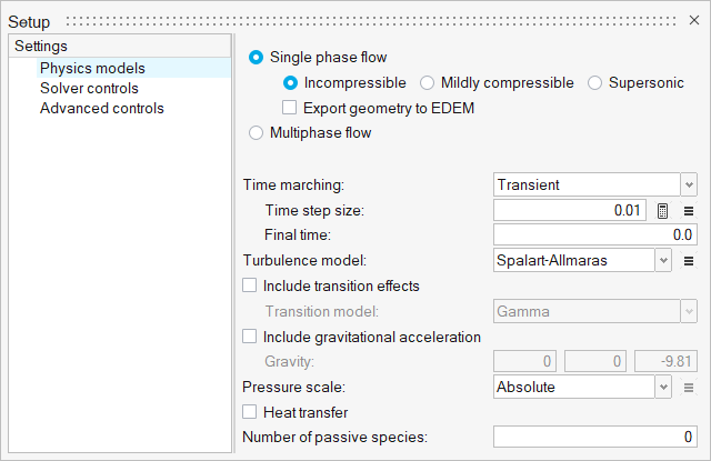
Figure 6. -
Click the Solver controls setting.
- Set the Minimum stagger iterations to 3.
- Set the Maximum stagger iterations to 20.
- Set the Transient maximum steps to 300.
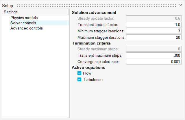
Figure 7.
Create a Multiplier Function
The force acting on the beam, due to the flow, will be ramped gradually over the first few time steps. After these first few time steps, the complete force from the fluid will be transferred to the beam without any ramping. This will be achieved using a Multiplier Function. In the next few steps you will create a linear multiplier function which will later be assigned as a force multiplier function for load acting on the beam.
-
From the Flow ribbon, click the arrow next to the
Setup tool set, then select Multipliers.
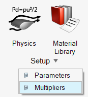
Figure 8.The Multiplier Library opens. -
Click
 to add a new
multiplier.
to add a new
multiplier.
-
Enter the table values according to the figure below.
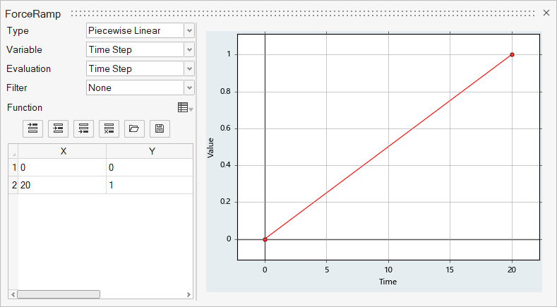
Figure 9.
Assign Material Properties
-
From the Flow ribbon, click the Material tool.

Figure 10. -
Select Water from the drop-down in the microdialog.
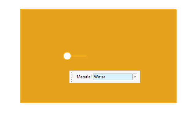
Figure 11. -
On the guide bar, click
 to execute
the command and exit the tool.
to execute
the command and exit the tool.
Assign the Flow Boundary Conditions
-
From the Flow ribbon, click the Constant tool.

Figure 12. -
In the microdialog, choose
Cartesian for the inflow velocity type and set X
velocity to 10.
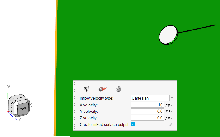
Figure 13. -
Click the Turbulence tab in the microdialog. Choose Direct for the
Turbulence input type and set Eddy viscosity to
1e-5.

Figure 14. -
Click
 on the guide bar.
-
Click the Outlet tool.

Figure 15. -
In the microdialog, verify that both the static
pressure and the pressure loss factor are set to 0.

Figure 16. -
Click on the guide bar.
-
Click the Slip tool.

Figure 17. -
Select the right-most face on the negative z-axis, as shown in the figure
below.
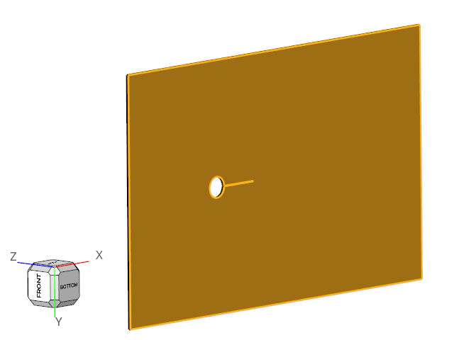
Figure 18. -
On the guide bar, click
 to execute the command and remain in the
tool.
to execute the command and remain in the
tool.
-
Click
 on the guide bar.
-
Select the right-most face on the positive y-axis, as shown in the figure
below.
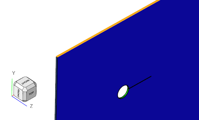
Figure 19. -
Click on the guide bar.
-
Click on the guide bar.
-
Click the No Slip tool.

Figure 20. -
Select the cylinder face, as shown in the figure below.

Figure 21. -
Click on the guide bar.
Set Up Motion
Define the Mesh Motion Type
-
From the Motion ribbon, click the Settings tool.
Figure 22.The Setup dialog opens. -
Activate Scale fields and select
ForceRamp for Multiplier function.
This will gradually ramp up the forces transmitted from the external code over the first few steps as specified by the multiplier function (20 time steps in this case).
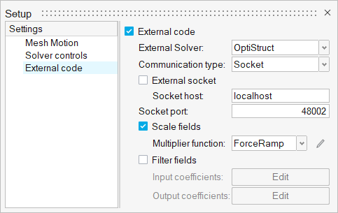
Figure 23.
Define the Mesh Displacement Boundary Conditions
-
From the Motion ribbon, click the External
Surface tool.

Figure 24. -
In the microdialog, select
Factor for the Gap method and set Gap factor to
0.
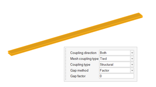
Figure 25. -
Click on the guide bar.
-
Click the Planar Slip
tool.

Figure 26. -
Select the right-most face on the negative z-axis, as shown in the figure
below
Figure 27. -
Click on the guide bar.
-
Click on the guide bar.
Define Time History Output Points
Time History Output commands enable you to extract the nodal solution at any point within the domain. In this simulation, it would be interesting to observe the displacement at the tip of the cantilever beam.
-
Form the Solution ribbon, click the body of the
Probe tool.

Figure 28. -
In the microdialog, set the Point Radius to
0.01.
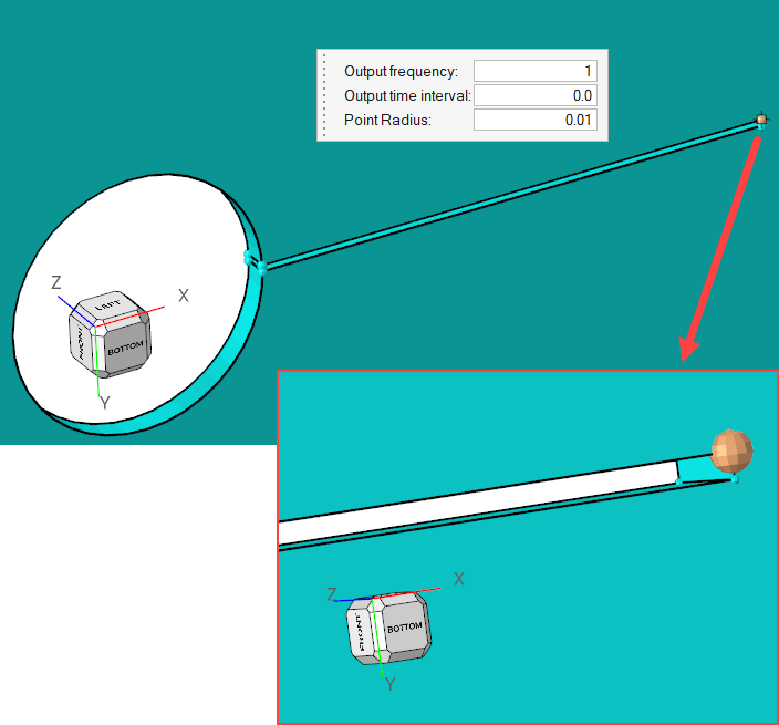
Figure 29. -
Click on the guide bar.
Define Nodal Outputs
The nodal output command specifies the nodal output parameters; for instance, output frequency, number of saved states, and so on.
-
From the Solution ribbon, click the Field tool.

Figure 30.The Field Output dialog opens. -
Under solution variables:
- Activate Write initial conditions.
- Activate Write results at time step interval.
- Set the Time step interval to 2.
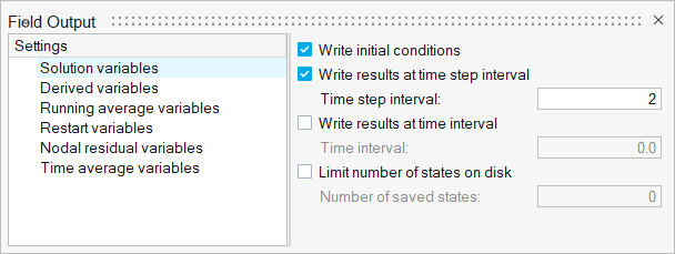
Figure 31.
Run OptiStruct
-
Click
 next to Input file(s).
-
Activate Use solver control.
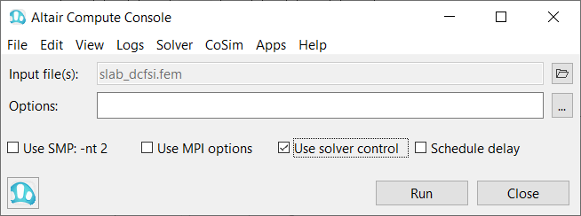
Figure 32.
Run AcuSolve
-
From the Solution ribbon, click the Run tool.

Figure 33. -
Leave the remaining options as default and click
Run to launch AcuSolve.
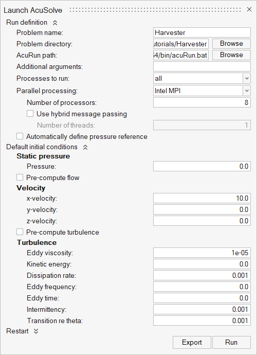
Figure 34. -
Right-click on the solver job in the Run Status dialog and
select View log file.
As the solution progresses, progress is reported in this window.
When AcuSolve is started, it will listen to the socket port specified while setting up the external code coupling for an initial communication from OptiStruct. You must make sure to start the OptiStruct run which will initialize the socket port for communication. Once the connection is established, the solvers will alternatively send and receive data through the simulation steps.
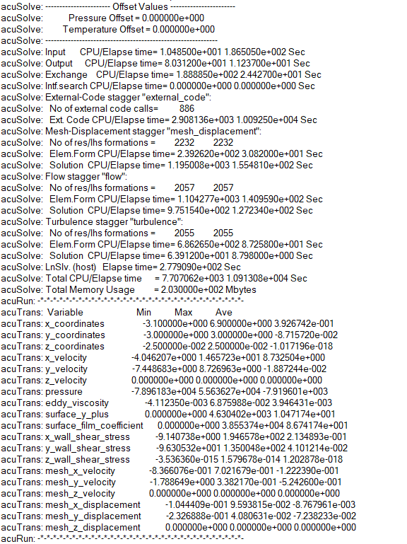
Figure 35.
Plot Time History
-
In the Plot Utility dialog, click to
create a new plot.
-
Under the Y-Axis heading, click the arrow besides Run
Data and select Time History.
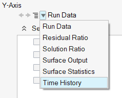
Figure 36. -
Select Node 1.
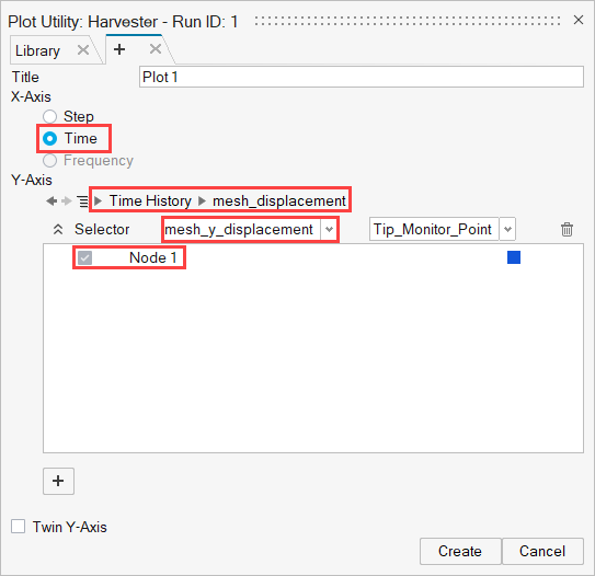
Figure 37. -
Click Create.
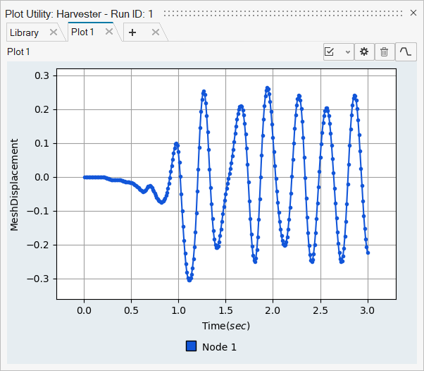
Figure 38. Mesh_y_displacement plot at beam tipThe plot above shows the displacement of the tip of the beam due to the fluid forces as the beam interacts with the flow.
Post-Process the Results with HW-CFD Post
-
Click the Bottom face on the View Cube to align the
model.
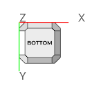
Figure 39. -
Move the slide bar at the bottom of the modeling window
to 74/151.

Figure 40. -
Activate the Legend toggle and click
 to refresh the legend.
-
Click
 and set the Colormap Name to Rainbow
Uniform.
and set the Colormap Name to Rainbow
Uniform.
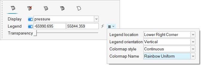
Figure 41. -
Click on the guide bar.
-
Click
 on the Animation toolbar to view a live animation
of the flow.
on the Animation toolbar to view a live animation
of the flow.
Figure 42. -
Save the animation.
- Go to .
-
Click
 and uncheck Include mouse
cursor.
and uncheck Include mouse
cursor.
- Set the frame rate to 24 and select GIF as the video setting.
-
Click
 on the toolbar then drag over the area you
want to record.
on the toolbar then drag over the area you
want to record.
-
Click
 to begin recording and the same icon to
stop recording.
to begin recording and the same icon to
stop recording.
- Name the file and save it.
Summary
In this HyperWorks CFD tutorial, you successfully set up and solved an FSI problem using the Direct Coupling, or DC-FSI approach. DC-FSI approach is a co-simulation approach where both the structural and the fluid solvers run simultaneously, and exchange information at each time step of the simulation. The fluid solver passes the flow and pressure information to the structural solver, which are used to determine the displacements in the structure. The structural solver then passes the displacement information to the fluid solver, which then recalculates the flow and pressure field. Both the solvers thus update and exchange the results of the simulation to achieve the solution. You started the tutorial by creating a database in HyperWorks CFD and setting up the basic simulation parameters. Then, you defined the parameters for setting up the connection between HyperWorks CFD and the structural solver, and generated a solution with co-simulation. Results were post-processed in HyperWorks CFD, where you generated an animation of the beam’s displacement as it interacted with the fluid flow.