HG-1050: Mouse Over - Inspect Mode
In this tutorial, you will learn how to utilize Inspect Mode.
- Inspect mode, which increases the screen area of the plot.
- Pre-highlight plot attributes (curves, legends, axes, and headers/footers) in gold when you move the mouse pointer over them.
- Display data point markers on a pre-highlighted curve.
- Highlight curves when selected from the Plot Browser, even when the curve is not in the active window. You can select one curve only from the Plot Browser or multiple curves; either way they are highlighted in gold in the plot(s).
- Use Inspect mode with multiple axes.
- Click the Build Plots icon,

- From the menu bar, select
This panel allows you to construct multiple curves and plots from a single data file. Curves can be overlaid in a single window or each curve can be assigned to a new window.
Open the nodout File
- From File menu, select to clear all contents in the HyperGraph 2D session.
-
Verify XY Plot is selected from the plot type menu,
 .
.
-
Click the Build Plots icon,
 .
.
-
Click the Open File button,
 , and select the nodout file,
located in the ../plotting/dyna/ folder.
, and select the nodout file,
located in the ../plotting/dyna/ folder.
Plot the Curves
-
Select option C and click
OK.
The following plots are displayed in the graphics area.
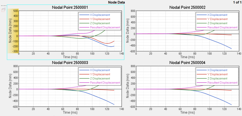 Figure 1.
Use Inspect Mode to Enlarge the Plot and Display Data Point Values
-
In the top-left plot, double-click in the plot area to enlarge the plot.
Double-clicking on an empty space in the plot (not on an entity) increases the screen area of the plot by hiding the panels and any other windows on the page. This is referred to as the Inspect Mode. In this case, since the plot was part of a multi-window layout, the other windows are also hidden so that the entire plot area is available for the plot that you selected.
Double-click in the white space of the plot again to reduce its size and go back to the four-window layout. However, for this step, leave the plot in its enlarged state.
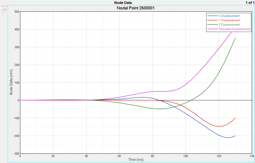 Figure 2.
 -
When you move the mouse over a curve before clicking on it, it is highlighted
in yellow, similar to the non-inspect mode.
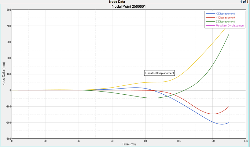 Figure 3.
 -
Click on the purple curve.
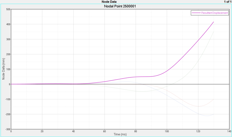
The curve becomes active. It displays its original color and the other curves become transparent.
Figure 4. -
Drag the mouse pointer along the curve to display the values of each point
along the curve.
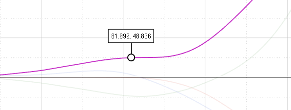 Figure 5.
 HyperGraph 2D only displays the value of the data points on a curve when the overlap is less than 50%. If it is more than that, only one value at a time is displayed.
-
Move the mouse pointer over the other transparent curves.
Note: They are highlighted in full color.
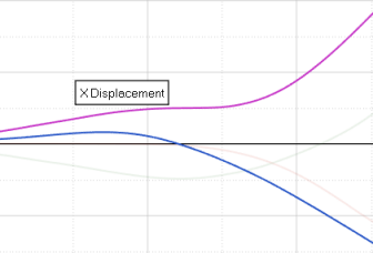 Figure 6.
 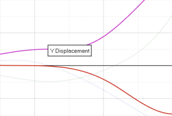 Figure 7.
 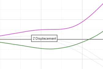 Figure 8.
 -
Click on the blue curve to make it active. The other three curves are now
transparent.
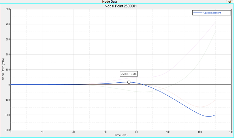 Figure 9.
 -
From the Plot Browser, you can select curves for multiple
plots even if they aren't in the active plot (the active plot is surrounded by a
blue border). The selected curves are highlighted in yellow.
In the image below, the curves selected from the Plot Browser (in blue) are highlighted in yellow in each of the four plots on the right. The active plot is displayed on the top-left and is surrounded by the blue rectangle.
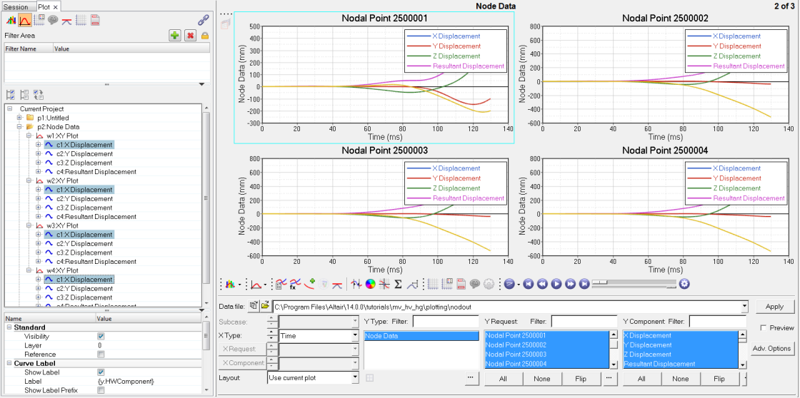 Figure 10.
Legend Handling
-
Click the Add Page icon,
 .
.
-
Click Apply.
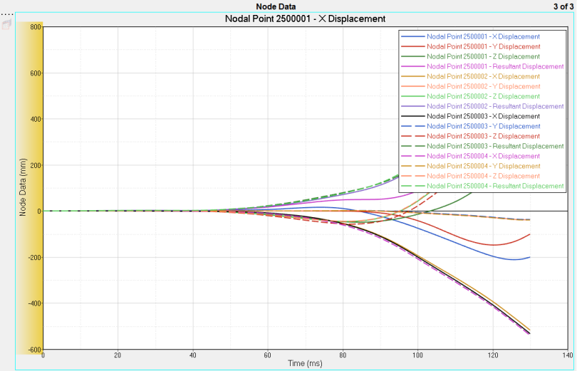 Figure 11.
 -
Click on any curve in the plot.
Note: When the curve is selected and active, the legend only displays the selected curve.
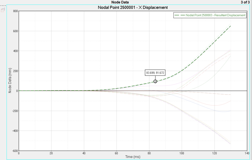 Figure 12.
Inspect Mode and Multiple Axes
-
Click the Add Page icon, .
-
Notice there are three axes:
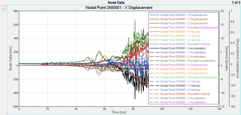 Figure 13.
 -
Click on any axis.
Note: When you click on an axis, you can only highlight the curves that belong to that axis.
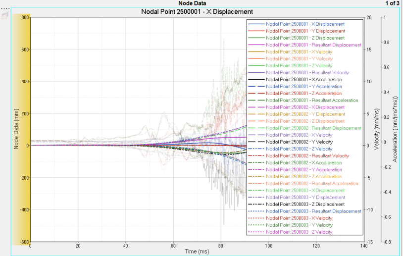 Figure 14.
 -
If you click the curve first, the axis automatically highlights. In the image
below, the curve selected belongs to the Acceleration axis.
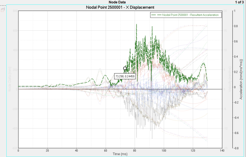 Figure 15.