Input Variable Properties

In the Define Input Variables step, various input variable properties can be modified from the Bounds, Modes, and Distributions tabs.

Bounds

Lower bound: Lower limit of the variable range to be studied.
Nominal: Default value of the variable if deactivated; also serves as the initial value in an Optimization.
Upper bound: Upper limit of the variable range to be studied.

Data Type

Real: Variable stored as a real valued floating point number, for example 1.0.
Integer: Variable stored as an integer, for example 1.0.
String: Variable stored as a character without any numeric meaning, for example one.

Mode

Continuous: Input variable that can take any value between the lower and upper bounds, for example 1 < x < 2.
Discrete: Input variable that can take values from an orderable finite list of numeric values, for example x = 0.1, 0.2, 0.3, or 0.4.
Categorical: Input variable that can take values from a non-orderable finite list of values, for example x = red, green, blue.

Distribution Role

Design: Variable that is deterministic and has no uncertainty associated with its value.
Random Parameter: Variable that is probabilistic, but is not controllable by design; for example wind speeds or temperature.
Design with Random: Variable that is probabilistic, but is controllable by design; for example thickness or radius.
Note: In a Stochastic approach, setting Distribution Role to Design with Random will use truncation sampling, in which any samples outside the Lower and Upper bounds are ignored.

Distribution

Input variables can be characterized statistically using various statistical distributions. An input variable, when used in a statistical sense, is termed as a random variable. In ordinary usage, the term "random variable" indicates that the value this variable will take is unknown, but in a statistical sense, it is precisely known what values this variable will take and the probability associated with that value.

Input variables exhibit different properties depending on the parameter they represent. Some variables may be symmetric about the mean value, while others may be skewed towards either the left or right. Some variables may be bounded on either side or unbounded.

The first categorization of random variables is whether the variable is continuous or discrete. A random variable is considered continuous if it can assume any value in a given interval. A random variable is termed discrete if it can only assume a finite set of values within a given interval.

Normal (CoV or Variance): Use to approximate many phenomenons in nature.

$f (x) = \frac{1}{\sqrt{2 Π σ^{2}}} e^{\frac{- {(x - μ)}^{2}}{2 σ^{2}}}$

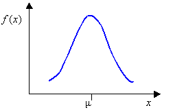
where $μ$ is the mean and $σ$ is the standard deviation.
Figure 1.; In HyperStudy a normal distribution can be defined using mean, $μ$ and variance, $σ^{2}$ or using mean, $μ$ and coefficient of variance (CoV), $σ$ / $μ$ .; Variance is the second statistical moment and measures the spread of a distribution. CoV measures the relative spread of a distribution. The higher the CoV, the higher the variability.
Uniform: Use when all values between the minimum and maximum are equally likely, such as a number from a random number generator.

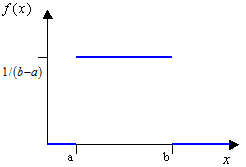
$\begin{array}{l} f (x) = {\begin{matrix} \begin{matrix} \frac{1}{b - a} \\ 0 \end{matrix} & \begin{array}{l} i f a \leq x \leq b \\ o t h e r w i s e \end{array} \end{matrix} \\ F (x) = {\begin{matrix} \frac{\begin{matrix} 0 \\ x - 1 \end{matrix}}{\begin{matrix} b - a \\ 1 \end{matrix}} & \begin{array}{l} i f x < a \\ i f a \leq x \leq b \\ i f x > b \end{array} \end{matrix} \end{array}$

where $a$ and $b$ are end points.
Figure 2.
Triangular: Use when the only known information is the minimum, the most likely, and the maximum values.

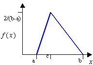
$f (x) = {| \begin{matrix} \frac{2 (x - a)}{(b - a) (c - a)} & i f a \leq x \leq c \\ \frac{2 (b - x)}{(b - a) (b - c)} & i f c \leq x \leq b \\ 0 & o t h e r w i s e \end{matrix}$

$F (x) = {\begin{matrix} 0 & i f x < a \\ \frac{{(x - a)}^{1}}{(b - a) (c - a)} & i f a \leq x \leq c \\ 1 - \frac{{(b - x)}^{1}}{(b - a) (b - c)} & i f c < x \leq b \\ 1 & i f b < x \end{matrix}$

where $a$ , $b$ , and $c$ are the end points and the mode.
Figure 3.
Exponential: Use to describe the amount of time between occurrences, mean time between failures.

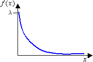
$\begin{array}{l} f (x) = {\begin{array}{l} λ e^{- λ x} & x \geq 0, \\ 0 & x < 0. \end{array} \\ F (x) = {\begin{array}{l} 1 - e^{- λ x} & x \geq 0, \\ 0 & x < 0. \end{array} \end{array}$

where $λ$ is the scale parameter.
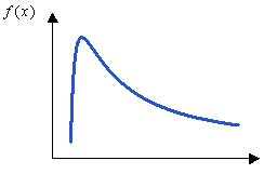
Figure 4.
Weibull: Principal applications are situations involving wear, fatigue and failure, failure rates, life-time expectancies.

$f (x) = {\begin{matrix} {α β^{- α} x^{α - 1} e}^{- {(\frac{x}{β})}^{α}} & i f x > 0 \\ 0 & o t h e r w i s e \end{matrix}$

$F (x) = {\begin{matrix} 1 - e^{- {(\frac{x}{β})}^{α}} & i f x > 0 \\ 0 & o t h e r w i s e \end{matrix}$

where $α$ and $β$ are shape and scale parameters which enable it to be adjusted to desired fatigue or reliability laws.
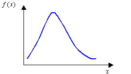
Figure 5.
Log Normal: Use in risk analyses.

$f (x) = \frac{1}{x s \sqrt{2 π}} e^{\frac{- {(1 n x - m)}^{2}}{2 s^{2}}}$

where $m$ and $s$ are location and scale.
Figure 6.
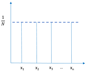
Uniform Discrete: Use when you have discrete (numeric or string) variables that take values which are equally likely.; Possible numeric values are 1, 2, 3, or 4; each are equally likely.; Possible string variables are orange, green, red, or blue; each are equally likely.; $f (x) = \frac{1}{N} \forall x \in {x_{1}, x_{2}, ... x_{n}}$
Figure 7.