HS-1705: Simple Fit Study
Learn how to set up a space filling DOE study, and then set up a Fit.
Before you begin, complete HS-1700: Simple DOE Study or import the HS-1700.hstx archive
file, available in <hst.zip>/HS-1705/.
Run Doe
-
Add a DOE.
- In the Explorer, right-click and select Add from the context menu.
- In the Add dialog, select DOE and click OK.
-
Define specifications.
- Go to the step.
- In the work area, set the Mode to Hammersley.
- Click Apply.
-
Evaluate tasks.
- Go to the step.
-
View a plot which illustrates the dependency between Area 2 and Response 1 and
Response 2.
-
Compare the scatter plots to determine if the runs are distributed
homogeneously throughout the design space.
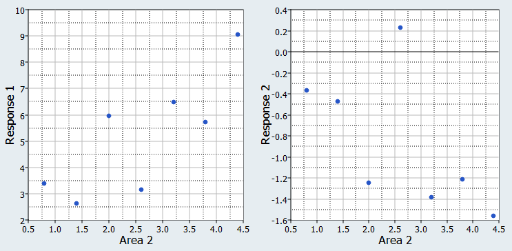
Figure 1.
-
Compare the scatter plots to determine if the runs are distributed
homogeneously throughout the design space.
Run Fit
-
Import matrix.
- Go to the step.
- Click Add Matrix.
- In the work area, set Matrix Source to Doe 2 (doe_2).
- Click Apply.

Figure 2. -
Define specifications.
- In the work area, Fit Type column, select Least Squares Regression (LSR) for both output responses.
- Click Apply.
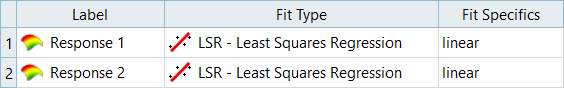
Figure 3. -
Post process results.
-
Click the Diagnostics tab and review the overall
Fit quality.
Several measures are shown to indicate the relative quality of the Fit. The R-Square value can be interpreted as the percentage of variance in the data that can be explained by the Fit.
For Response_1, the Fit captures 100% of the data variance; this makes sense as Response_1 is actually a linear function so the first order regression matches the actual data with no error. For Response_2, it is shown below that the Fit explains about 90% of the variance.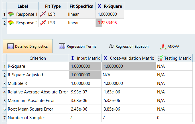
Figure 4.
-
Click the Diagnostics tab and review the overall
Fit quality.