Steps in AcuSolve

Introduction

In this section, the steps involved in AcuSolve to import the file of Joule losses volume densities are given.

Steps in AcuSolve

The steps in AcuSolve to import the losses file are described below with screen shots.

Define AcuSolve project with:
- Geometry
- Mesh
- Physics
Import the Joule losses file:
Tools > Electromagnetics Manager

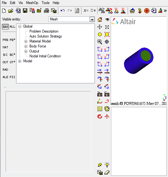
The following box is opened:
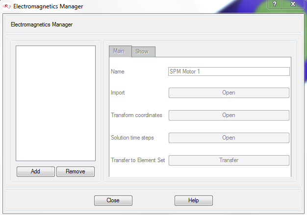In the Electromagnetics Manager box, follow the steps:
- Click on Add button
- Change the name from SPM Motor 1 to Flux
- In the Import field click Open, then select the Flux losses file to import and click Open
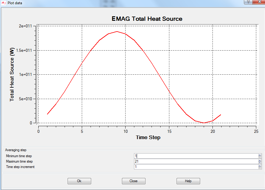
- This will open the EMAG Total Heat Source window showing the total heat source vs time step plot and the averaging step data at the bottom of plot as shown in below figure. Select the right averaging time steps and click on OK
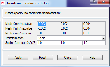
- In Transform coordinates click Open
- This will open the Transform Coordinates Dialog box showing the coordinate transformation in all three x,y,z directions. Click Apply and then Close button.
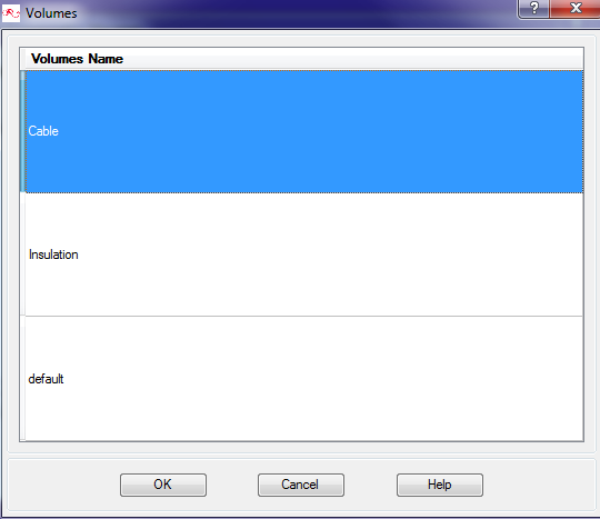
- Click Transfer in the Transfer to Element Set field. This will open the Volumes dialog box. Here we select the “Cable” volume group from the dialog box and we click OK
- Click Close to exit the Electromagnetics Manager
- In order to confirm whether the heat source is correctly applied to the Cable volume group we can check the Element Set under Volumes in the data tree manager as follows.
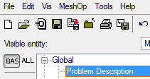
  - Switch to BAS in the data tree manager
  - Expand Cable group under Volumes model tree
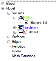
  - Double click on Element Set to open Element Set detail panel
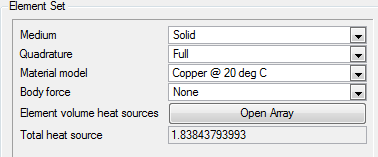
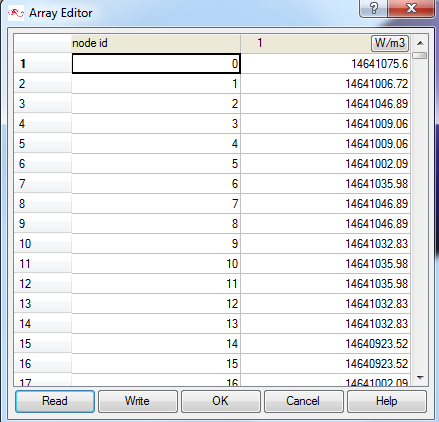
  - Click Open Array in the field Element volume heat sources. You can see that the heat source is updated for the node id as shown below
- Click OK to close the Array Editor.
- You can also see the Total heat source. Here it is updated to 1.838
Run AcuSolve simulation