Steps in Flux to export the losses
Introduction
In this section, the steps involved in Flux to generate the file of Joule losses volume densities are given.
General presentation
- Steady state AC magnetic application
- Transient application:
In this case, it is possible to export Joule losses densities time evolution or mean values on one period.
- 2D Plane
- 2D axisymmetric
- 3D
Study case
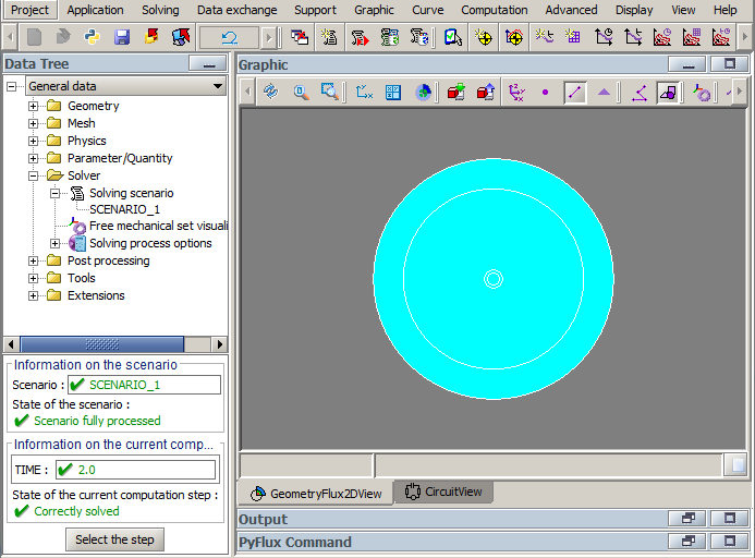
The studied case in this document is a cable heating by Joule losses.
In this document, the case is simulated in Flux 2D plane transient magnetic application. The time evolution of Joule losses is exported.Import/Export context
The Import/Export context is dedicated to all couplings with other software, including the coupling with AcuSolve.
It replaces the old export to AcuSolve available through the menu:
The Import/Export context gives much more possibilities and options to couple with AcuSolve.
Steps in Flux
- Define Flux project with:Remark: if the project solving scenario contains lot of time steps (or parameter steps), it is advised to solve after the step 6 to earn computation time.
- Geometry
- Mesh
- Physics
- Solving
-
Open Import/Export context :
- Before solving
- After solving
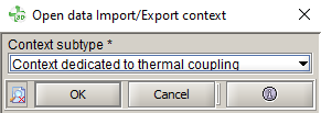
- Before solving
- Select the thermal coupling context:
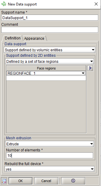
- The first step in the Import/Export context is to create the data support:
The data support creation box is opened
- In the data support creation box, select:
- The data support type:
Usually to compute Joule losses support defined by volumic entities is chosen.
It corresponds to “volume” entities in 3D (volumes, volume regions, etc.) and “surface” entities in 2D (faces, face regions, etc.).
- Choose the support defined by 2D entities:
The most communly we select the face regions.
- Select the support entities:
Here in the list of face regions, we select the “CABLE” region.
- In 2D, in order to export the data in 3D, user has to select Extrude in the Mesh extrusion field, and enter the number of elements in the extrusion depth, for example 10.
- Select Yes if you want to rebuild the full
device when you have symmetries or periodicities.
- The data support type:
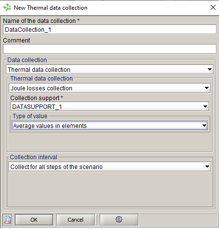
- The second step in the Import/Export context is to create the thermal data collection:
The thermal data collection creation box is opened
- In the data collection creation box, select:
- The thermal data collection Joule losses collection
- The collection support DATASUPPORT_1 created before
- The type of value Average values in elements
Remark: other types won’t be compatible to export to AcuSolve
- The collection interval:
It is advised to choose collect for all steps of the scenario. In steady state AC this choice has no influence. In transient the computation will be done on all scenario steps.
- Now the data collection has to be evaluated:
The thermal data collection is computed
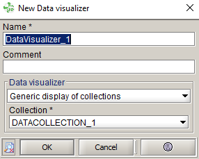
- Before exporting, the results can be visualised in Flux for verification :
The Data visualizer box is opened
- In the data visualizer box, select:
- The collection DATACOLLECTION_1 created
previously
The Joule losses are visualized: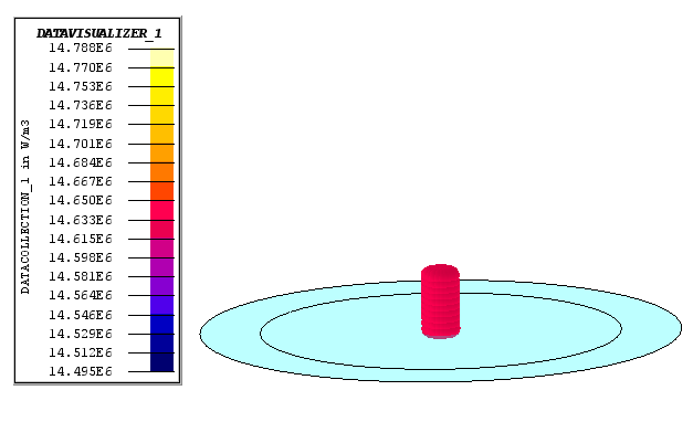
- The collection DATACOLLECTION_1 created
previously
- The last step is to export the results:
The Data collection export box is opened
- In the data collection export box:
- Select the collection DATACOLLECTION_1 created previously
- Write the File name
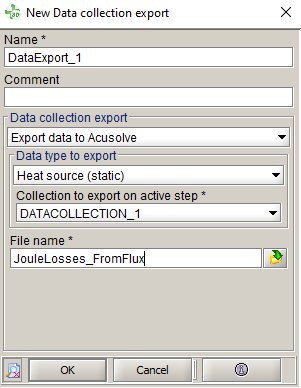
The file is exported