Improved coil conductor regions in 3D with relaxed geometrical constraints
Suppression of geometrical constraints on the shapes of volumes integrating coil conductor regions in 3D due to a new method for evaluating the current density.
Overview
In previous versions of Flux 3D, the creation of volume regions of type coil conductor region was subjected to significant geometrical constraints. The geometry (i.e., the volumes, faces, lines and points assigned to such a region) was required to have a uniform cross section, as if the faces belonging to the input electric terminal had been extruded along the current path described by the winding (図 1).
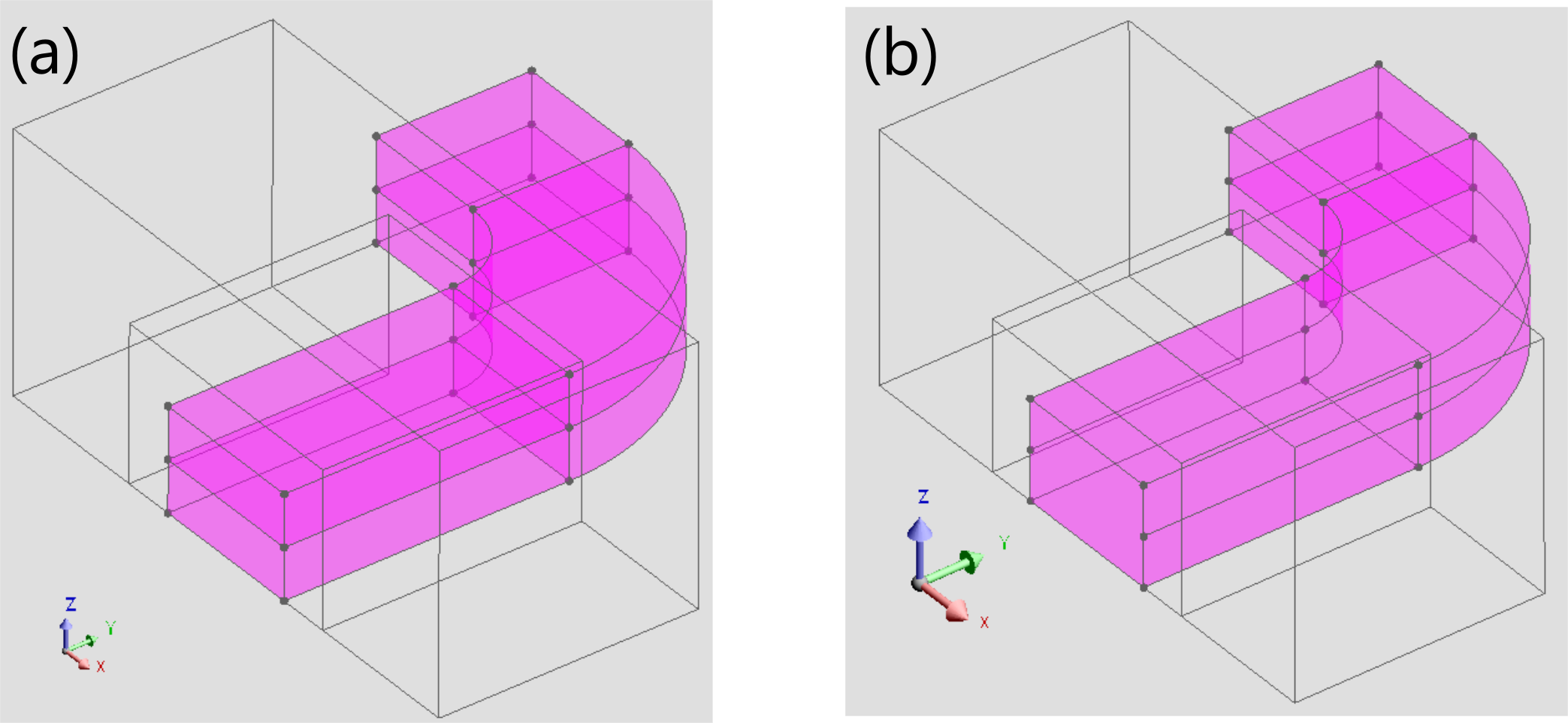
図 1. Representation in Flux 3D of one eighth of a coil, with three symmetries. While the geometry of the coil in part (a) satisfies the constraints imposed to coil conductor regions in the previous versions of Flux 3D, the alternative geometry in part (b) does not. However, the geometry in (b) may now be assigned to a coil conductor region in Flux 2021.1.
To circumvent these limitations, Flux’s latest release provides a new method to compute the current density J in coil conductor regions in 3D. Consequently, several geometrical restrictions were lifted, and now in version 2021.1 a coil conductor region may:
- be assigned to a geometry part imported into a Flux project from a CAD file,
- contain “parasite” points and lines anywhere in its volumes,
- share a common interface with other parts of the simulated device (e.g., the magnetic circuit of the coil),
- have input and output terminals with different numbers of faces,
- have cross sections (i.e., the sections orthogonal to the current flow) with varying shapes between the input and output terminals.
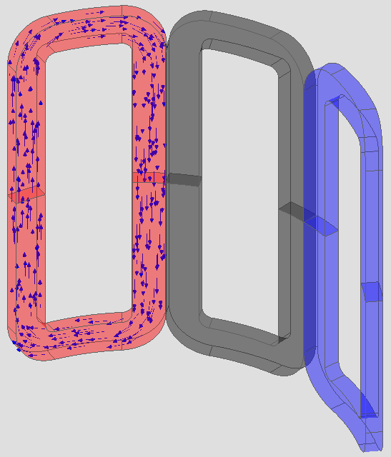
図 2. Evaluation of the current flow in three coil conductor regions with the latest Flux release. In previous versions, the volumes assigned those regions in the example would have to be described in a more intrincated way (i.e., by decomposing the coil in additional volumes) to avoid geometrical constraints. The arrows represent the current density J in the left coil.
Availability for coil conductor region subtypes
This new feature is available in Flux 3D only for the following subtypes of coil conductor regions:
- Coil conductor region without losses or
- Coil conductor region with losses and simplified geometrical description.
In these cases, the following restriction applies: the area of the section orthogonal to the direction of the current density must not significantly change between the input and output terminals. On the other hand, the shape of the cross-section is allowed to change.
For the third subtype Coil conductor region with losses and detailed geometrical description, the geometrical constraints from the previous versions remain.
For further information on the new subtypes of coil conductor regions mentioned above, please refer to the following section of this release note: New GUI and user guide for coil modeling.
Choosing the new method of evaluation of the current density by adjusting the solving process options
Flux needs to evaluate the current density J in coil conductor regions at certain points during the solving process and while the user is post-processing the solution.
The new method to compute this current density leading to coil conductor regions subjected to lighter geometrical constraints may be selected from a new list of solving options called Method for the computation of J in coil conductor regions in 3D (available from the Solving menu, with the following choices: ). The user may choose one of the following options from that list:
- Automatically specified method: the default selection
- Analytical method or by interpolation from lines: the approach available in previous versions, which may only be applied to volumes subjected to significant geometrical constraints
- Method with electric conduction resolution (with finite element method) + uniform J norm: the new approach introduced in Flux 2021.1
These options are explained in the next three paragraphs.
Analytical method or by interpolation from lines
In this approach, the geometry of the coil conductor region must have a constant cross-section, as if the faces of the input electric terminal had been extruded along the current path towards the output terminal (as depicted in 図 3).
Under such circumstances, the current density is computed with simple analytical formulas or by an interpolation method, depending on the nature of the geometrical entities (i.e., if they were created by the user through Flux internal modeler or if they were imported from a CAD file).
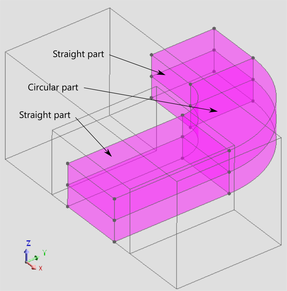
図 3. Geometry with straight and circular parts
Method with electric conduction resolution (with finite element method)+ uniform J norm
The steps of this new method are explained below:
- At the beginning of the solving process, a finite element computation of an electric conduction problem is performed in each Coil conductor region. The electric scalar potential V is used as state variable and a resistivity of 1 Ω.m is admitted. The values of V at each node are stored.
- During the solving process or while in post-processing, the current density J is computed at a point from V, with formula J = -grad V. Then the direction of J is kept, but its norm is adjusted. It results uniform in the whole region, with a value that depends on the section areas of the electric terminals, the number of turns of the coil, the number of wires in parallel and the coefficient for coils flux computation related to the existence of symmetries or periodicities.
Automatically specified method
With this solving option:
- In the cases of a Coil conductor region without losses or
of a Coil conductor region with losses and simplified geometrical
description.
- the software verifies if the geometry of the coil conductor region is compatible with the Analytical method or by interpolation from lines.
- If it is compatible, this Analytical method or by interpolation from lines is used.
- Otherwise, the Method with electric conduction resolution + uniform J norm is used.
- For a Coil conductor region with losses and detailed geometrical description, the Analytical method or by interpolation from lines is used.
- the coil conductor region subtype and
- the compatibility of the geometry with the approach Analytical method or by interpolation from lines,
| Type of volume region | Geometry compatible with the "Analytical method or by interpolation from lines" | Actual method used for the computation of J |
|---|---|---|
|
Coil conductor region without losses or Coil conductor region with losses and simplified geometrical description |
Yes | Analytical method or by interpolation from lines |
| No | "Method with electric conduction resolution (with finite element method) + uniform J norm | |
| Coil conductor region with losses and detailed geometrical description | Yes | Analytical method or by interpolation from lines |
| No | Flux displays an error message during resolution. |
Modification in the workflow for orienting coil conductor regions
The following two commands:
- Orient wires of coil conductor region (completion mode), or
- Orient wires of coil conductor region (modify mode)
are still required to assign the electric terminals to a coil conductor region in 3D.
However, the workflow for orienting the current sense in the coil has slightly changed in the case of coil conductor regions with External terminals because of this new feature. Previously, Flux asked the user to select only the faces of the input terminal and automatically determined the faces of the output terminal. In this new version, however, Flux will ask the user to select the faces of the output terminal as well.
The workflow for orienting the current sense in the coil remains unchanged in the case of a coil conductor region with Internal terminals: the faces of the input terminal and of the output terminal are coincident, and thus Flux only asks for the faces on the input terminal and for a line defining the current sense.Backward compatibility: opening of a Flux project saved in a previous version of the software
For projects solved with a previous version of the software, the approach Analytical method or by interpolation from lines is employed when the user chooses to continue with the solution of a partially treated scenario.
For unsolved projects, the Automatically specified method is used.