List of Flux 2021.1 new features
a short description of each new features and improvements of this version.
New features dealing with Environment
| New features | Description |
|---|---|
| Dynamic Memory Performance |
The first version of Dynamic memory management has been integrated in Flux 2020. By default, User (or static) memory was activated in supervisor options. Since two versions we continued to work on critical algorithms to improve the robustness and performance of Flux with the Dynamic memory mode. Thanks to these improvements, the performance obtained with dynamic memory is now close to the user mode. We advise you to use Flux with dynamic memory without parallel computing (several Flux process on a same machine). With parallel computing, we advise the User mode. Indeed, in dynamic memory mode each process queries the OS for dynamic allocation. There is therefore a risk of saturation of the OS. We are continuing our work to improve performances, in particular to improve the use of dynamic memory with parallel computing for future versions. |
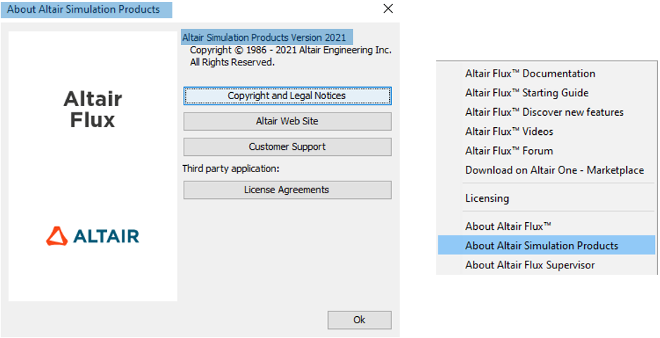
| New branding | HyperWorks term is
replaced by Altair Simulation Products
注: the link with the Altair Web Site button has
been also changed: https://www.altair.com/simulation-driven-design//
|
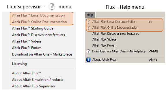
| New features about documentation |
The new features about the documentation are:
|
New features dealing with Physics
| New features | Description |
|---|---|
| New GUI and user guide for coil modeling |
In order to simplify the creation and to clarify the underlying
models of Coil conductor regions in Flux,
the GUI (i.e., the dialog box) of this
type of region has been renewed. This new
GUI merges two "legacy" regions, namely:
Further details on this new GUI, on backward compatibility issues and on a new section of the user guide dedicated to the modeling of coils and windings are presented in this page. |
| Improved coil conductor regions in 3D with relaxed geometrical constraints |
In previous versions of Flux 3D, the creation of volume regions of type "coil conductor region" was subjected to significant geometrical constraints. The geometry (i.e., the volumes, faces, lines and points assigned to such a region) was required to have a uniform cross section, as if the faces belonging to the input electric terminal had been extruded along the current path described by the winding. To circumvent these limitations, Flux’s latest release provides a new method to compute the current density in coil conductor regions. Consequently, several geometrical restrictions were lifted, and now in version 2021.1 a coil conductor region may:
For further details on this new method and on its availability in Flux, please refer to the following release note chapter. The user guide will be updated with information on this subject in an upcoming version of Flux. |
New macros
| New macros | Description |
|---|---|
| CreatePark_dq_From_abc |
Create dq parameter from abc component using Park transformation. Input:
Output:
|
|
ExportForcePerToothTo CSVSingleFile |
Macro for exporting force by tooth in general-pourpose CSV format. Useful for 2D models of rotating machines. Previous steps to call the macro:
Inputs:
Output: A CSV file. It contains a table with nine columns: number of case, mean speed, mean torque, number of the tooth, tooth coordinates (x,y), frequency/time, normal force and tangential force |
| CreateLookUpTableFrom TMProjectDQLight |
Create look up table from TM project of Flux dq, Ld, Lq and torque versus Id, Iq and rotor position. Input:
Output: result OML file with name created from the initial file (*_res.oml) and with more data such as phase resistance, end winding inductance, electric period and initial rotor position with possibility to display in Compose |
| Analyse Hysteresis Material |
This macro represents the hysteresis cycle of a material, which magnetic property is described according with Jyles-Atherton or Preisach models. It will launch a parametric study, varying maximum magnetic field (Hmax) to represent several hysteresis cycles. Warning: When this macro is launched, the current Flux project will be closed and a new one is launched. To save the initial project previously is highly recommended. Inputs:
Outputs:
|
New/Updated examples
As a reminder, all examples are accessible via the Flux supervisor, in the context of Open an example.
| New/Updated examples | Description |
|---|---|
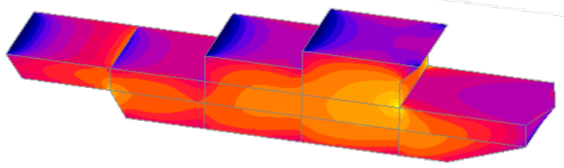
| Magnetic signature of a
vessel 3D Application Note New |
This example explains how to simulate the
magnetic signature of a ship.
 |
| DC_Motor 2D Application Note Update |
The studied device is a DC motor. Python and documentation have been updated to unload the overlay after the creation. 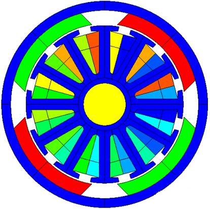 |
| Switch Reluctance
Machine 2D Application Note Update |
This simulation presents the electromagnetic modeling of Flux switching permanent magnet machine using Flux 2D and HyperStudy to maximize the efficiency. 3 new cases have been added: Example 4: Design Optimization in HyperStudyA study to optimize the design of Flux Switching Motor to increase efficiency. 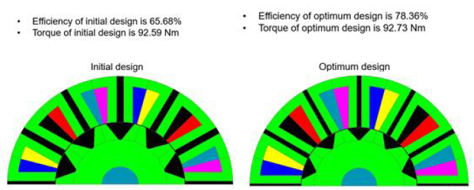 A study to perform Thermal analysis on Flux Switching Motor. Thermal Analysis is performed to obtain Heat Transfer Coefficients of surfaces of motor for Natural Convection. 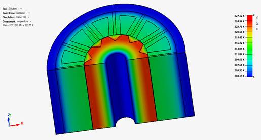 A study to perform Thermal analysis on Flux Switching Motor in Flux to obtain temperature distribution in motor. Average losses in the model are obtained and Heat sources are calculated. Using the heat source and boundary conditions, the Maximum temperature in motor is obtained for inner wall temperatures from 303.15 K to 373.15 K. 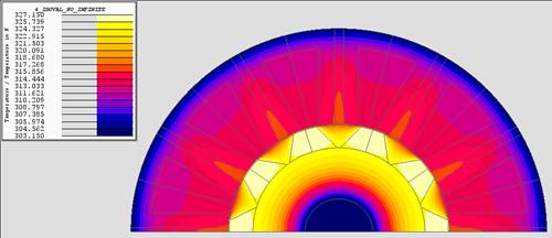 |
| Brushless IPM
Motor 2D Technical Tutorial Update |
The study proposed in the "Brushless IPM motor tutorial" is a study of a motor designed for hybrid electric vehicle traction/generation. New macro CreateLookUpTableFromTMProjectDQLight.PFM. has been added in this version, and this example has been updated with this macro. This update allows to obtain same results between Flux and FluxMotor. 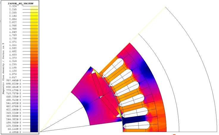 |