OS-T: 6010 Multiaxial Fatigue Analysis (Damage Calculation) using S-N Approach
In Multiaxial Fatigue Analysis, OptiStruct uses the stress tensor directly to calculate damage.
Multiaxial Fatigue Analysis theories are based on assumption that stress is in the plane-stress state. In other words, only free surfaces of structures are of interest in Multiaxial Fatigue Analysis in OptiStruct.
For solid elements, a shell skin is automatically generated by OptiStruct, shell elements are used as-is. Multiaxial Fatigue Analysis features are activated by setting MAXLFAT=YES on the FATPARM Bulk Data Entry.
Further for the S-N approach, the Goodman and the Findley models are used to check the damage caused by the tensile and the shear cracks.
The following files found in the optistruct.zip file are needed to perform this tutorial. Refer to Access the Model Files.
ctrlarm.fem, load1.csv and load2.csv
or
A copy of the model files used in this tutorial are available on <install_directory>/tutorials/hwsolvers/optistruct/.
In this tutorial, a control arm loaded by brake force and vertical force is used, as shown in Figure 1. Two load time histories acquired for 2545 seconds with 1 HZ, shown in Figure 2 and Figure 3, are adopted. Because a crack always initiates from the surface, a skin meshed with shell elements is designed to cover the solid elements, which can improve the accuracy of calculation as well.
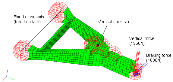
Figure 1. Control Arm for Fatigue Analysis Model
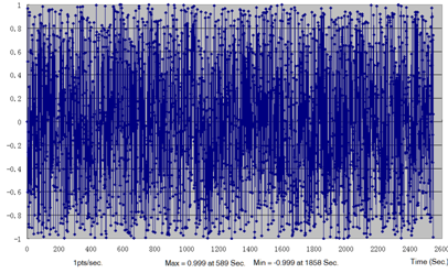
Figure 2. Load Time History for Vertical Force
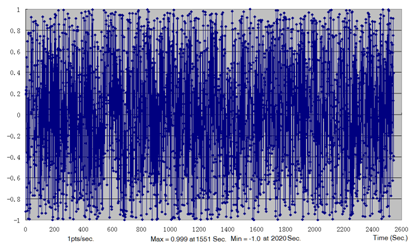
Figure 3. Load Time History for Braking Force
Launch HyperMesh and Set the OptiStruct User Profile
Import the Model
-
Select the Files icon
 .
A Select OptiStruct file browser opens.
.
A Select OptiStruct file browser opens. -
Click Import, then click Close to
close the Import tab.
The outline of the Fatigue Analysis setup to be achieved in the following steps.
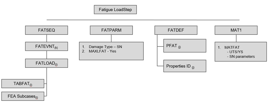
Figure 4. Fatigue Setup – MultiAxial SN
Set Up the Model
Define TABFAT Load Collector
Define FATLOAD Load Collector
- In the Model Browser, right-click and select .
- For Name, enter FATLOAD1.
- Click Color and select a color from the color palette.
- For Card Image, select FATLOAD.
- For TID(table ID), select table1 from the list of load collectors.
- For LCID (load case ID), select SUBCASE1 from the list of load steps.
- Set LDM (load magnitude) to 1.
- Set Scale to 3.0.
- Repeat the process to create another load collector named FATLOAD2 with FATLOAD Card Image and pointing to table2 and SUBCASE2.
- Set LDM to 1 and Scale to 3.0.
Define FATEVNT Load Collector
- In the Model Browser, right-click and select .
- For Name, enter FATEVENT.
- For Card Image, select FATEVNT.
- For FATEVNT_NUM_FLOAD, enter 2.
-
Click on the Table icon
 next to the Data field and select FATLOAD1 for FLOAD(1)
and FATLOAD2 for FLOAD(2) in the pop-out window.
next to the Data field and select FATLOAD1 for FLOAD(1)
and FATLOAD2 for FLOAD(2) in the pop-out window.
Define FATSEQ Load Collector
Define Fatigue Parameters
- In the Model Browser, right-click and select .
- For Name, enter fatparam.
- For Card Image, select FATPARM.
- Verify TYPE is set to SN.
- Set MAXLFAT to Yes for the multiaxial method.
- Set STRESSU to MPA (Stress Units).
- Set RAINFLOW RTYPE to LOAD.
Define Fatigue Material Properties
The material curve for the fatigue analysis can be defined on the MAT1 card.
Define PFAT Load Collector
- In the Model Browser, right-click and select .
- For Name, enter pfat.
- For Card Image, select PFAT.
- Set LAYER to TOP.
- Set FINISH to NONE.
- Set TRTMENT to NONE.
- Set Kf to 1.0.
Define FATDEF Load Collector
- In the Model Browser, right-click and select .
- For Name, enter fatdef.
- Set the Card Image to FATDEF.
- Activate PSOLID in the PTYPE Entity Editor.
- Edit FATDEF_PSOLID_NUMIDS to 2. The model contains 2 solid properties defined in the model.
-
Click on the Table icon
next to the Data field and select PSOLID_2 for PID(1),
pfat for PFATID(1) and
PSOLID_5 for PID(2) and pfat
for PFATID(1) in the pop-out window.
- Click Close.
Define the Fatigue Load Step
- In the Model Browser, right-click and select .
- For Name, enter Fatigue.
- Set the Analysis type to fatigue.
- For FATDEF, select fatdef.
- For FATPARM, select fatparam.
- For FATSEQ, select fatseq.
Submit the Job
Review the Results
-
On the Results toolbar, click
 to open the
Contour panel.
to open the
Contour panel.
-
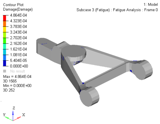 Figure 5. Elemental Life results indicating ~4500 cycles before the first
element fails
Figure 5. Elemental Life results indicating ~4500 cycles before the first
element fails