OS-T: 3000 Topography Optimization of a Plate Under Torsion
In this tutorial you will perform a topography optimization of a plate under torsion.
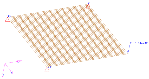
Figure 1. Finite Element Model of the Design Space with Loads and Constraints
A finite element model is loaded into HyperMesh. The constraints, load, material properties, and subcase (loadstep) of the model are already defined. Topography design variables and optimization parameters are defined and the OptiStruct software determines the optimal reinforcement patterns. The results are viewed as animations of the contours of shape changes of the design space. Finally, the use of the grouping patterns is shown; based on the shape changes suggested by OptiStruct, a possible pattern is chosen for ease of manufacturing.
- Objective
- Minimize nodal displacement at grid point where loading is applied.
- Design Variables
- Shape variables generated automatically on the designable space aligned with the elements normal.
Launch HyperMesh and Set the OptiStruct User Profile
Open the Model
Verify the Thickness of the Component
Set Up the Optimization
Define Topography Design Variables
For a topography optimization, a design space and a bead definition need to be defined.
Create Optimization Responses
- From the Analysis page, click optimization.
- Click Responses.
-
Create the displacement response.
- Click return to go back to the Optimization panel.
Define the Objective Function
- Click the objective panel.
- Verify that min is selected.
- Click response and select displace.
- Using the loadsteps selector, select torsion.
- Click create.
- Click return twice to exit the Optimization panel.
Run the Optimization
- torsion_plate.hgdata
- HyperGraph file containing data for the objective function, percent constraint violations, and constraint for each iteration.
- torsion_plate.hist
- The OptiStruct iteration history file containing the iteration history of the objective function and of the most violated constraint. Can be used for a xy plot of the iteration history.
- torsion_plate.html
- HTML report of the optimization, giving a summary of the problem formulation and the results from the final iteration.
- torsion_plate.oss
- OSSmooth file with a default density threshold of 0.3. You may edit the parameters in the file to obtain the desired results.
- torsion_plate.out
- OptiStruct output file containing specific information on the file setup, the setup of the optimization problem, estimates for the amount of RAM and disk space required for the run, information for all optimization iterations, and compute time information. Review this file for warnings and errors that are flagged from processing the torsion_plate.fem file.
- torsion_plate.sh
- Shape file for the final iteration. It contains the material density, void size parameters and void orientation angle for each element in the analysis. This file may be used to restart a run.
- torsion_plate.stat
- Contains information about the CPU time used for the complete run and also the break-up of the CPU time for reading the input deck, assembly, analysis, convergence, and so on.
- torsion_plate_des.h3d
- HyperView binary results file that contain optimization results.
- torsion_plate_s#.h3d
- HyperView binary results file that contains from linear static analysis, and so on.
- torsion_plate.grid
- An OptiStruct file where the perturbed grid data is written.
View the Results
Shape contour information is output from OptiStruct for all iterations. In addition, Displacement and Stress results are output for the first and last iteration by default. This section describes how to view those results using HyperView.
View a Static Plot of Shape Contours
-
On the Results toolbar, click
 to open the
Contour panel.
to open the
Contour panel.
-
Set Result type to Shape Change (v) and
Mag.
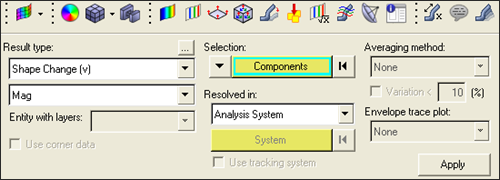
Figure 2. -
On the Animation toolbar, click
 to choose the last iteration from the
Simulation list.
A deformed plate appears.
to choose the last iteration from the
Simulation list.
A deformed plate appears.
Is the max= field showing 4.0e + 00?
In this case, it is. If it is not, your optimization has not progressed far enough. Decrease the OBJTOL parameter (set in the opti control panel on the optimization panel). This value, 4.0e+00, comes from the draw height defined earlier.
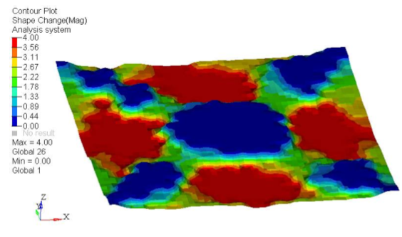
Figure 3. Contour Plot . showing the reinforcement pattern at the last iteration (converged solution)
View a Transient Animation of the Shape Contour Changes
-
From the Animation toolbar, set the animation mode to
 (Transient).
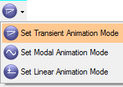
Figure 4. - Click
 to start the animation.
 -
Click
 to open the Animation Controls panel.
- Click
 to pause the animation.
View the Deformed Structure
The displacement and stress results from the first and last iterations (default) are given in the torsion_plate_s1.h3d file.
-
In the top, right of the application, click
 to go
to the next page.
This page has the subcase information from the torsion_plate_s1.h3d file.
to go
to the next page.
This page has the subcase information from the torsion_plate_s1.h3d file. -
On the Results toolbar, click
 to
open the Deformed panel.
to
open the Deformed panel.
-
In the Results Browser, select the first iteration
(Iteration 0).
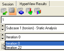
Figure 5. -
On the Animation toolbar, set the animation mode to
 (Linear Static).
- Click to start the animation.
- Click to go to the Animation Controls panel.
- Click
 to stop the animation.
 -
On the Page Controls toolbar, click
 to
delete the HyperView page.
to
delete the HyperView page.
Add Pattern Grouping Constraints
Pattern grouping will be added as a constraint for manufacturability.
A possible pattern, suggested by the static contour plot obtained in the previous exercise, is to use channels parallel to a diagonal. In this example, you choose the diagonal emerging from the node where the load is applied.
-
Select nodes.
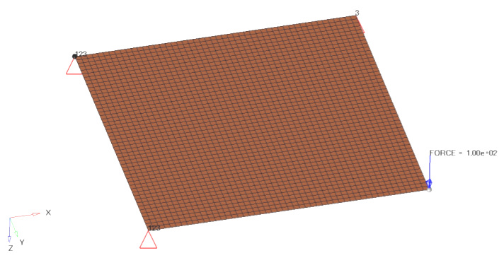
Figure 6. Pattern Grouping Node Location
Run the Optimization
View the new results as before. Also check the objective value for the zero-th and last iteration in the .out file. How does the final value for the objective compare to the final value obtained using 'none' option for pattern grouping?
View a Static Plot of Shape Contours
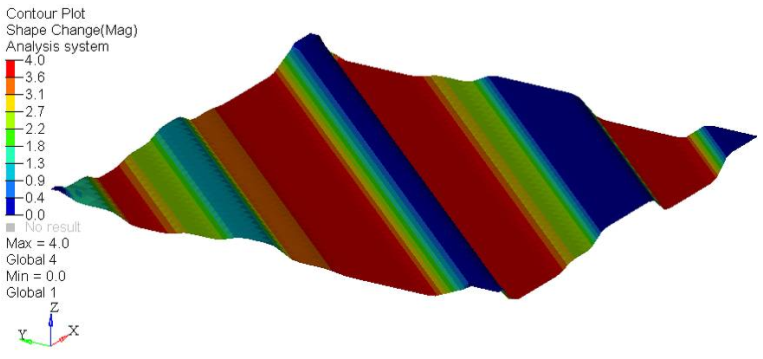
Figure 7. Contour Plot Showing the Reinforcement Pattern . with pattern grouping constraint at the last iteration.