OS-T: 5100 Stress Response based on Neuber Correction Method
The tutorial demonstrates Neuber shape optimization to reduce the stress concentration at the fillet regions by changing its shape.
- Set up the objective, constraints and design variables in HyperMesh
- Submit the job in OptiStruct
- View results in HyperView
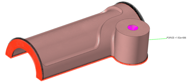
Figure 1. Model and Loading Description
- Objective
- Minimize the change in mass.
- Constraints
- Minimize the static stress to a value less than 330 MPa using Neuber correction method
- Design Variables
- Shape design variables.
Launch HyperMesh and Set the OptiStruct User Profile
Open the Model
Set Up the Model
Create Property
Here you will assign the property, as the Valve is a solid part.
- In the Model Browser, right-click and select .
- For Name, enter PSOLID.
- For Card Image, select PSOLID.
- For Material, select Aluminum.
- From the Model Browser, Component folder, right-click on Valve and assign the property PSOLID.
Create FORCE Load Collector
First you will isolate the component and then apply the force.
-
Assign the values, as shown in the image.
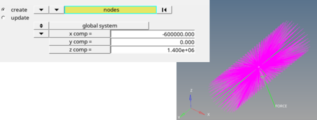
Figure 2. Apply Force
Create SPC Load Collector
-
Similarly, select the other side faces of the Valve and
select only dof1 and dof2.
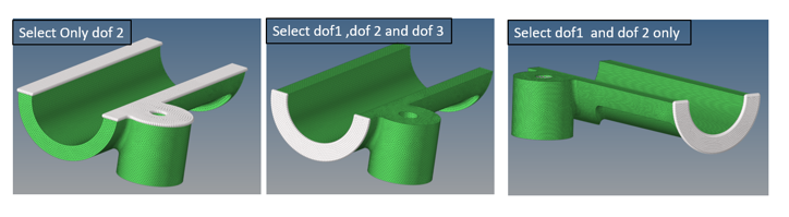
Figure 3. Apply Constraints
Create Load Steps
Create Design Equations
-
In the edit equation field, enter
delta(x)=x-9.892e-02.
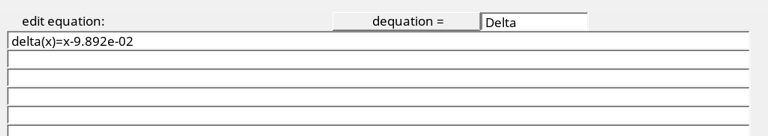
Figure 4. Design Equation -
Select , select valve and click
calculate.
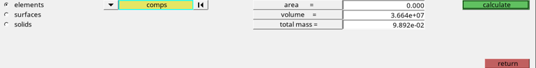
Figure 5. Mass of the Valve
Create Shape Optimization Design Variables
-
Click create and return.
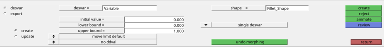
Figure 6. Create Design VariablesNote: Potential variation in the shape of the Valve is increased in the fillet radius.
Create Optimization Responses
Create Mass Response Type
-
In the drop-down, select response type as
mass and click return.

Figure 7. Mass Response
Create Static Stress Response Type
-
Select neuber correction, as shown in the image.
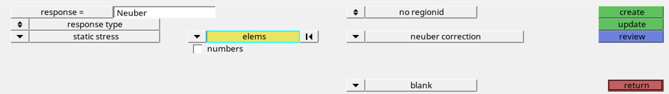
Figure 8. Static Stress Response
Create Function Response Type
-
Expand Response List and select Optiresponse as the
Mass.
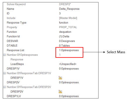
Figure 9. Function Response TypeNote: To create change in mass response, Function response is used here.
Create Design Constraints
- Click the dconstraints panel.
- In the constraint= field, enter Constraints.
- Click response type and select neuber, which is a static stress response type.
- Select loadstep 1 - Static.
- Select upper bound and enter a value of 330.
Define the Objective Function
- Click the objective panel.
- Verify that min is selected.
- Click response type and select Delta_Response.
- Click Create.
Define the SHAPE Card
Only displacement and stress results are available in the .h3d file by default. In order to look at displacement/stress results on top of a shape change that was applied to the model in HyperView, a SHAPE card needs to be defined.
- From the Analysis page, click the control cards panel.
- In the Card Image dialog, click SHAPE.
- Set FORMAT to H3D.
- Set TYPE to ALL.
- Set OPTION to ALL.
- Click return twice to go back to the main menu.
Run the Optimization
View the Results
The following steps demonstrate how to review the contour plot with the optimized shape in HyperView.
It is helpful to view the deformed shape, stresses in the model using Neuber correction method .
-
In the Results tab, select Iteration 23, the last
iteration.
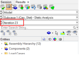
Figure 10. Iterations Selection -
On the Results toolbar, click
 to open the
Contour panel.
to open the
Contour panel.
-
Set Result type to Shape change (v) and click
Apply to contour the elements.
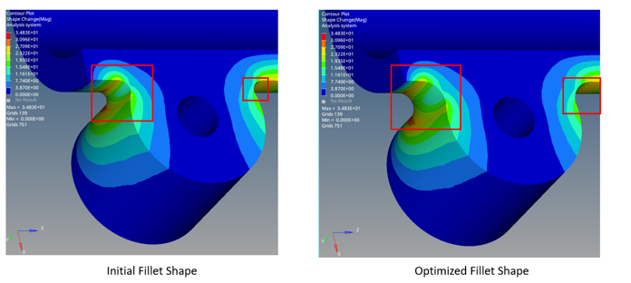
Figure 11. Shape Change Results -
Click Apply.
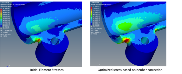
Figure 12. Element Stress Results -
Select <filename>_hist.mwv to view the change in mass
and the optimized mass after changing the shape.
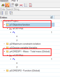
Figure 13. Session Plot Results -
View the plot results for objective function and total mass.
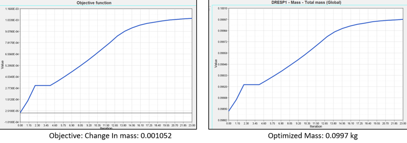
Figure 14. Objective Function and Total Mass Plot