Concrete and Rock Materials
In Radioss these materials can be used to represent rock or concrete materials.
These materials use a Drücker–Prager yield criterion1, which is a pressure-dependent model for determining whether a material has failed or undergone plastic yielding.
Concrete Material (/MAT/LAW10 and /MAT/LAW21)
Drücker-Prager Yield Criteria
- Second stress invariant (von Mises stress) of the deviatoric part of the stress and .
- First stress invariant (hydrostatic pressure).
- In a uniaxial test.
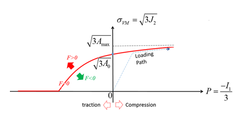
Figure 1. Drücker-Prager yield criteria
- If , the material is under yield surface and is in the elastic region.
- If , and the material is at the yield surface.
- If , and the material is past the yield surface and has failed.
- If , , which is the von Mises criterion.
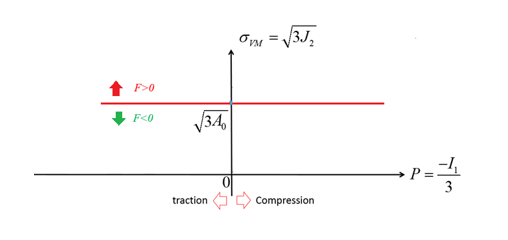
Figure 2.
Pressure Computation
- If , the pressure is and the pressure limit is .
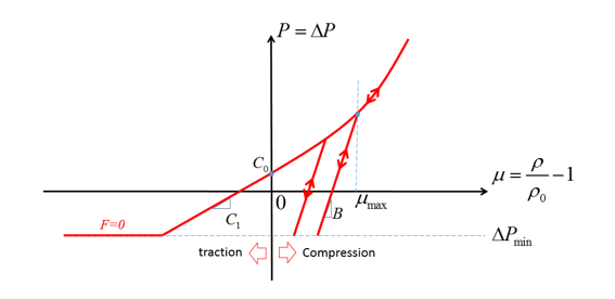
Figure 3. Pressure curve without external pressure - If , the pressure is shifted by , then and the pressure limit is .
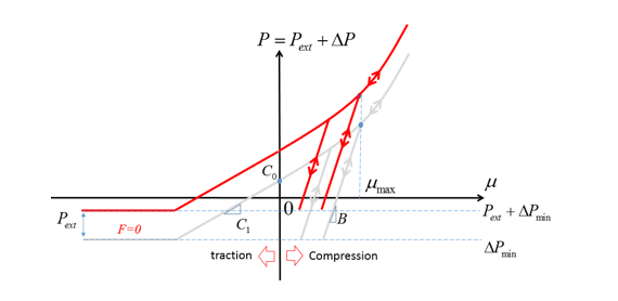
Figure 4. Pressure curve with external pressure
- In traction or tension the pressure is linear and limited by .
- In compression the pressure is nonlinear also limited by .
The only difference between the material laws is that in LAW10 the material constants are used to describe the pressure versus volumetric strain ( curve). In LAW21 you can describe this curve via function input fct_IDf.
Load and Unload
- In Tension ()
- For LAW10, linear loading and unloading with (Figure 3).
- For LAW21, loading is defined using the input function fct_IDf and linear unloading with .
- In Compression (), for both LAW10 and LAW21:
- If neither B and
are defined, the loading and unloading path
are identical.

Figure 5. Identical loading and unloading for LAW10 and LAW21 - If either B or
is defined:
- If only B is defined, is the volumetric strain where the tangent of curve is equal to B with .
- If only
is defined, then B is the tangent
of curve at
. The loading and unloading in
compression is:
- If , loading and unloading path are identical.
- If , loading and unloading
path are different, it is linear unloading with
slope B.
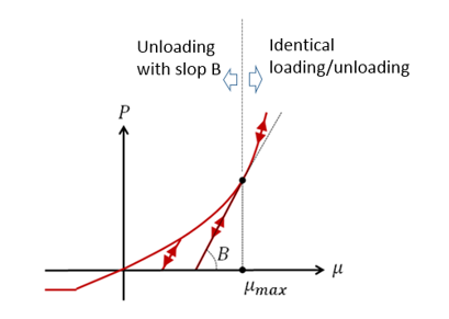
Figure 6. Different loading and unloading treatment for LAW10 and LAW21
- If neither B and
are defined, the loading and unloading path
are identical.
Concrete Material (/MAT/LAW24)
LAW24 uses a Drücker-Prager criteria with or without a cap in yield to model a reinforced concrete material. This material law assumes that the two failure mechanisms of the concrete material are tensile cracking and compressive crushing.
Concrete Tensile Behavior
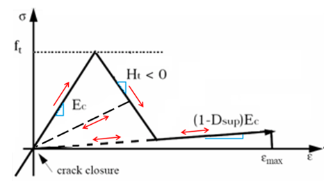
Figure 7. LAW24 Tensile Loading
In the initial very small elastic phase, the material has an elastic modulus Ec.
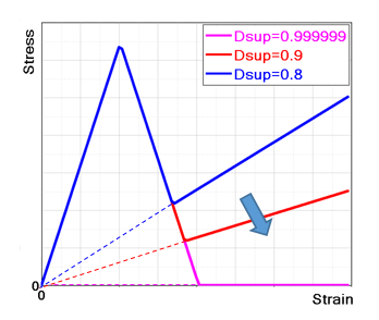
Figure 8. Maximum Damage Factor Effects
When there is crack closure, the concrete becomes elastic again, and the damage factor (for each direction) is conserved.
The bearing capacity of concrete in tensile is much lower than in compression. It is normally considered elastic when in tension.
It is recommended to choose a Dsup value close to 1 (default is 0.99999) in order to minimize the current stiffness at the end of the damage and consequently avoid residual stress in tension, which can become very high if the element is highly deformed due to tension. This will happen if the force causing the damage remains.
It is possible to adjust the Dsup (and Ht) in order to simulate and fit the behavior of concrete reinforced by fibers. The concrete material fails once it reaches the total failure strain .
Concrete Yield Surface in Compression
For concrete, the yield surface is the beginning of the plastic hardening zone which is between the failure surface, , and the yield surface.
- For Icap
=0 or 1 (without a cap in yield) the
yield curve is:
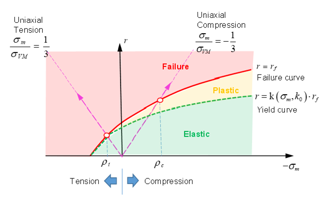
Figure 9. Drücker-Prager Criteria without a Cap in Yield - For Icap
=2 (with cap in yield) the yield is:
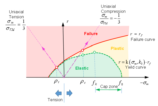
Figure 10. Drücker-Prager Criteria with Cap in Yield
The input parameter is the hydrostatic failure pressure in a uniaxial tension test and is the hydrostatic pressure by failure in a uniaxial compression test.
- When (in tension) the scale factor . In this case, the yield surface equals the
failure surface, .

Figure 11. Function in the Tension Zone - In the tension-compression region, , thenwith
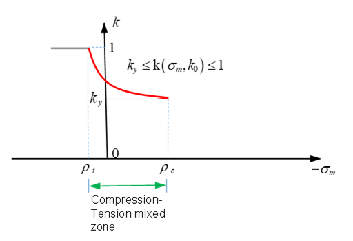
Figure 12. Function in the Compression-Tension Mixed Zone - The rest of the curve depends on the
Icap option and the
different scale factors used.
- For Icap
=0 or 1 and (in compression), then
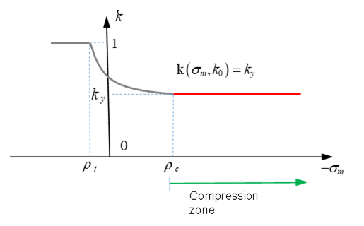
Figure 13. Function in the Compression Zone - For Icap
=2 (with cap in yield) and (in compression), then
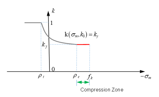
Figure 14. Function in Drücker-Prager Criteria without a Cap - In (in cap zone)with

Figure 15. Function in Drücker-Prager Criteria with a Cap
- For Icap
=0 or 1 and (in compression), then
The material constant should be . A higher value of results in a higher yield surface.
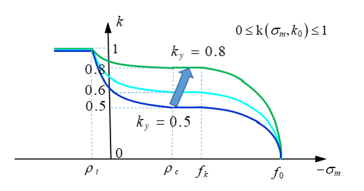
Figure 16. Affect of Different Function Values
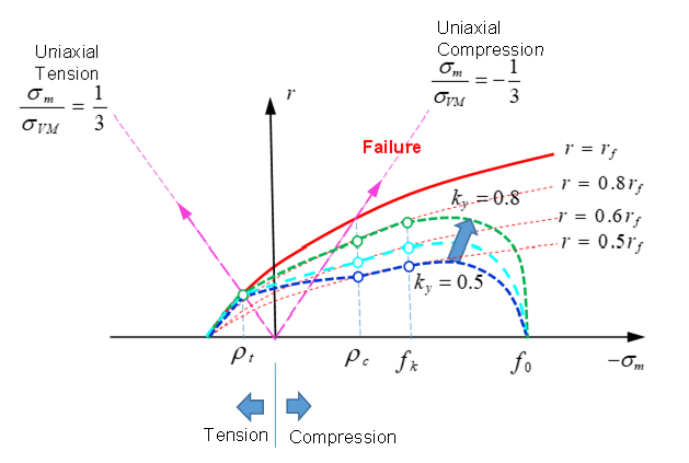
Figure 17. Drücker-Prager Criteria with Different Function Values
Concrete Plastic Flow Rule in Compression
- Plastic dilatancy.
- Governs the volumetric plastic flow.
- First stress invariant (hydrostatic pressure).
- If
- then, which means the material is in yield.
- If
- then, becomes negative is the cap region.
- If
- then, which means the material has failed.
The values of are used to describe the material beyond yield, but before failure. It is recommended to use -0.2 and -0.1 for in LAW24. If very small values of are used, there is no volumetric plasticity (no cap region).
Concrete Crushing Failure in Compression
- Uniaxial tension (triaxiality is 1/3)
- Uniaxial compression (triaxiality is -1/3)
- Biaxial compression (triaxiality is -2/3)
- Confined compression strength (tri-axial test)
- Under confined pressure
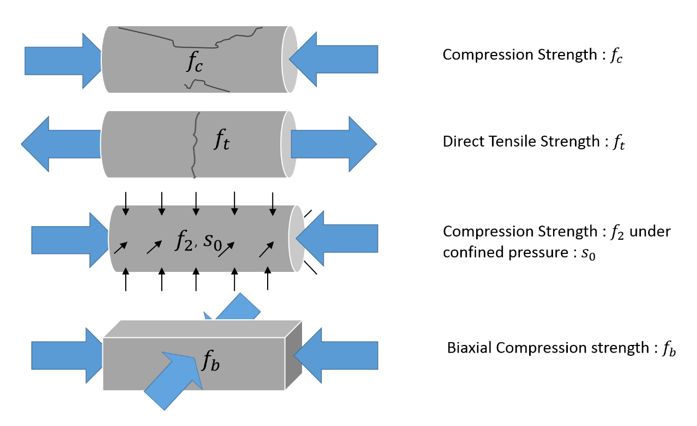
Figure 18. Failure Parameters that Fully Determine 3D Failure Envelope
| Load Type | Surface Point | Default Input | Criteria | Pressure | Lode Angle |
|---|---|---|---|---|---|
| Compression | Mandatory | ||||
| Direct Tensile | |||||
| Biaxial Compression | If
Icap =
1
If Icap = 2
|
||||
| Compression Strength under Confinement Pressure |
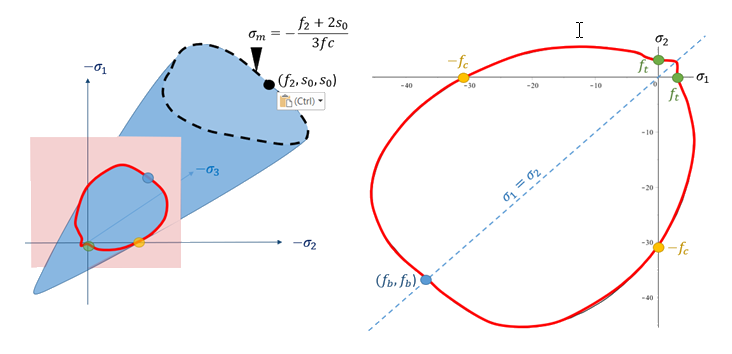
Figure 19. Trace of failure surface with planar stress plane
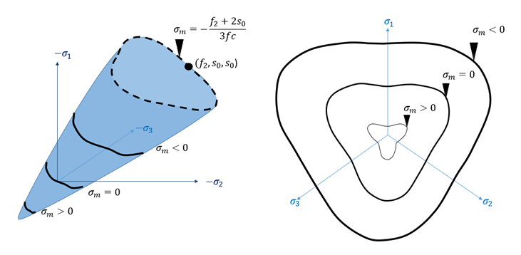
Figure 20. Failure trace with several cut plan which are normal to the hydrostatic axis
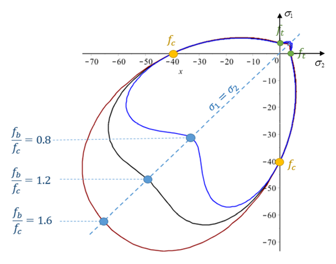
Figure 21. Influence of the biaxial compressive strength value with all other characteristic failure points fixed
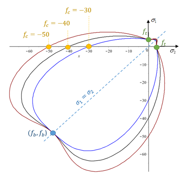
Figure 22. Influence of the compressive strength value with all other characteristic failure points fixed
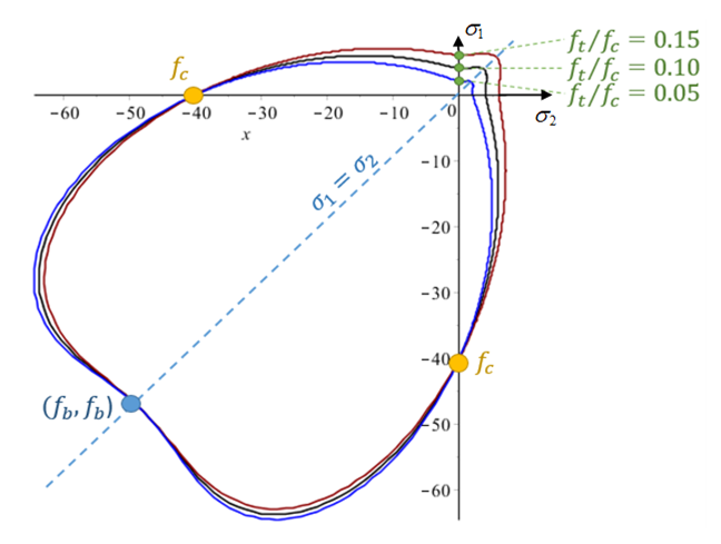
Figure 23. Influence of the tensile strength value with all other characteristic failure points fixed
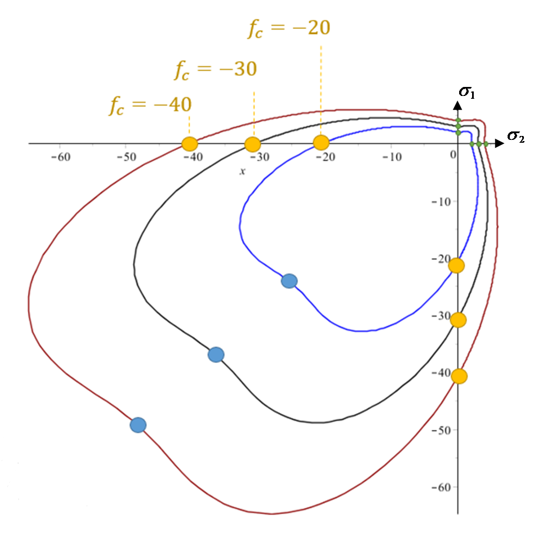
Figure 24. Influence of compressive strength value. All other ratios are fixed.
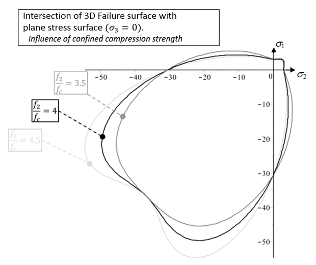
Figure 25. Failure envelope on the plane stress surface influenced by the triaxial failure point
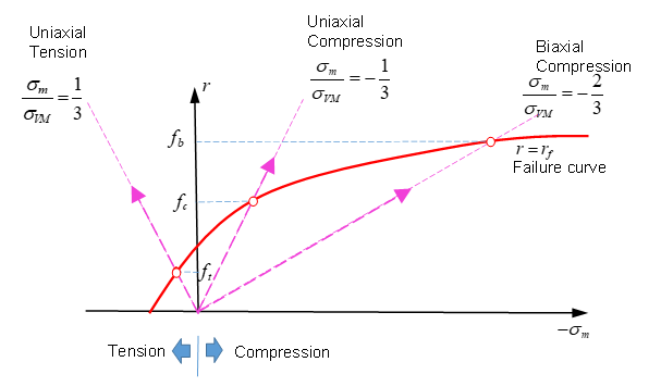
Figure 26. Different tests (uniaxial tension, uniaxial compression, and biaxial compression) to determine failure curve
Where the failure curve is defined using and is the mean stress (pressure), then and are the first and second stress invariants.
The material fails once it reaches the failure curve .
Concrete Reinforcement
- One way is to use beam or truss elements and connect them to the concrete with kinematic conditions.
- Another way is to use the parameters in LAW24 along with the orthotropic
solid property /PROP/TYPE6 to define the reinforced
direction. Parameters in LAW24 are used to define the
reinforcement cross-section area ratio to the whole concrete section area in
direction 1, 2, 3.
(13)
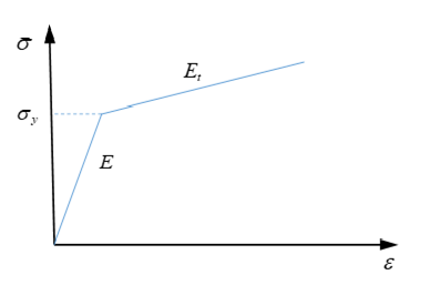
Figure 27. Stress-Strain Curve of Reinforcement (steel)
Concrete Material (/MAT/LAW81)
LAW81 can be used to model rock or concrete materials.
Drücker-Prager Yield Criteria
- von Mises stress with
- Pressure is defined as
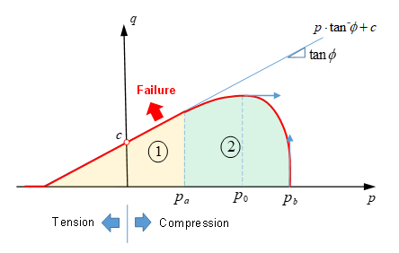
Figure 28. Yield Surface (LAW81)
- The linear part
 (), where the scale function is which leads to the von Mises stress being
linearly proportional to pressure:
(), where the scale function is which leads to the von Mises stress being
linearly proportional to pressure:(15) Where,- Cohesive and is the intercept of yield envelope with the shear strength.
- Angle of internal friction, which defines the slope of the yield envelope.
and are also used to define the Mohr-Coulomb yield surface. The Drücker-Prage yield surface is a smooth version of the Mohr-Coulomb yield surface.
- The second part
 () of the yield surface simulates a cap limit.
An increase of pressure in a rock or concrete material will increase the
yield of the material; but, if pressure increases enough, then the rock or
concrete material will be crushed. The Drücker-Prager model with the cap
limit can be used to model this behavior. The cap limit defined in part
and uses the scale
function:
() of the yield surface simulates a cap limit.
An increase of pressure in a rock or concrete material will increase the
yield of the material; but, if pressure increases enough, then the rock or
concrete material will be crushed. The Drücker-Prager model with the cap
limit can be used to model this behavior. The cap limit defined in part
and uses the scale
function:(16) The von Mises stress is:(17) Where,- Curve is defined using the fct_IDPb input
- Computed by Radioss using the input ratio value.
with .
Where, is the maximum point of yield curve, where
If , then and the yield function is then,
which means the material is crushed.
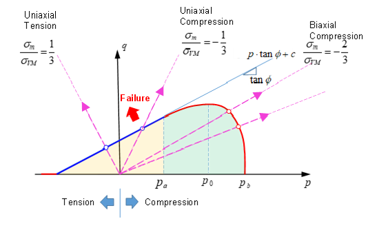
Figure 29. Yield Surface of LAW81 Showing Different Load Conditions
- if
- if
- if
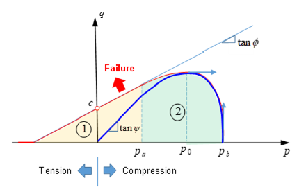
Figure 30. Yield Surface of LAW81 with Plastic Flow