Steps for iron losses computation on regions
This section describes the steps to carry out iron losses computation on regions:
-
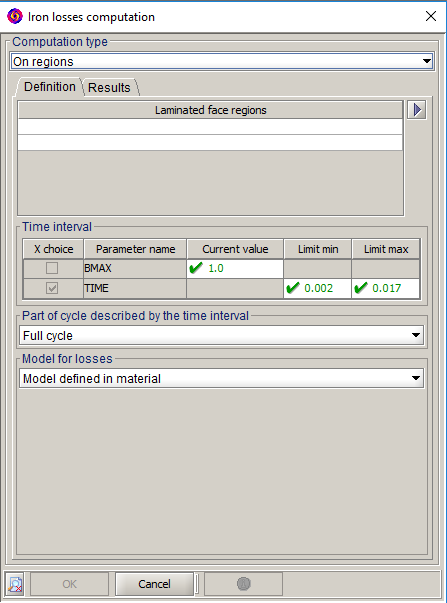
In Transient magnetic, define the time period selected in the previous step. The various possibilities are presented in the table below:
Choices Description Full cycle The user have to choose a full electrical period in the time step interval. A periodicity indicator is displayed in the result gui box of the iron losses.Note: The first two steps of the scenario are hidden as they cannot be selected for this computation.Half cycle (advanced mode) The user have to choose a half electrical period in the time step interval. A periodicity indicator is displayed in the result gui box of the iron losses.Note: The first two steps of the scenario are hidden as they cannot be selected for this computation.The rebuilded signal is antiperiodic. Note: Half cycle option can manage a signal with a DC component.
No cycle Flux does not take into consideration the period. Note: For the LS model, there is also a " hysteretical " transient for the first selected step, it appears because the point is living the B(H) solving curve (first magnetization curve, anhysteretic curve etc.) to match the rebuilded B(H') hysteresis loop during iron losses computation.