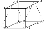
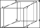
Hourglass Modes

Hourglass modes are element distortions that have zero strain energy. Thus, no stresses are created within the element. There are 12 hourglass modes for a brick element, 4 modes for each of the 3 coordinate directions.

Γ

represents the hourglass mode vector, as defined by Flanagan-Belytschko. ¹ They produce linear strain modes, which cannot be accounted for using a standard one point integration scheme.

Γ^{1} = (+ 1, - 1, + 1, - 1, + 1, - 1, + 1, - 1)

Γ^{2} = (+ 1, + 1, - 1, - 1, - 1, - 1, + 1, + 1)

Γ^{3} = (+ 1, - 1, - 1, + 1, - 1, + 1, + 1, - 1)

$Γ^{4} = (+ 1, - 1, + 1, - 1, - 1, + 1, - 1, + 1)$

To correct this phenomenon, it is necessary to introduce anti-hourglass forces and moments. Two possible formulations are presented hereafter.

Kosloff and Frasier Formulation

The Kosloff-Frasier hourglass formulation ² uses a simplified hourglass vector. The hourglass velocity rates are defined as:(1)

\frac{\partial q_{i}^{α}}{\partial t} = \sum_{I = 1}^{8} Γ_{I}^{α} \cdot v_{i I}

Where,

$Γ$: Non-orthogonal hourglass mode shape vector
$ν$: Node velocity vector
$i$: Direction index, running from 1 to 3
$I$: Node index, from 1 to 8
$α$: Hourglass mode index, from 1 to 4

This vector is not perfectly orthogonal to the rigid body and deformation modes.

All hourglass formulations except the physical stabilization formulation for solid elements in Radioss use a viscous damping technique. This allows the hourglass resisting forces to be given by:(2)

f_{i I}^{h g r} = \frac{1}{4} ρ c h {(\sqrt[3]{Ω})}^{2} \sum_{α} \frac{\partial q_{i}^{α}}{\partial t} \cdot Γ_{I}^{α}

Where,

$ρ$: Material density
$c$: Sound speed
$h$: Dimensional scaling coefficient defined in the input
$Ω$: Volume

Flanagan-Belytschko Formulation

In the Kosloff-Frasier formulation seen in Kosloff and Frasier Formulation, the hourglass base vector

Γ_{I}^{α}

is not perfectly orthogonal to the rigid body and deformation modes that are taken into account by the one point integration scheme. The mean stress/strain formulation of a one point integration scheme only considers a fully linear velocity field, so that the physical element modes generally contribute to the hourglass energy. To avoid this, the idea in the Flanagan-Belytschko formulation is to build an hourglass velocity field which always remains orthogonal to the physical element modes. This can be written as:(3)

v_{i I}^{H o u r} = v_{i I} - v_{i I}^{L i n}

The linear portion of the velocity field can be expanded to give:(4)

v_{i I}^{H o u r} = v_{i I} - (\bar{v_{i I}} + \frac{\partial v_{i I}}{\partial x_{j}} \cdot (x_{j} - \bar{x_{j}}))

Decomposition on the hourglass vectors base gives ¹:(5)

\frac{\partial q_{i}^{α}}{\partial t} = Γ_{I}^{α} \cdot v_{i I}^{H o u r} = (v_{i I} - \frac{\partial v_{i l}}{\partial x_{j}} \cdot x_{j}) \cdot Γ_{I}^{α}

Where,

$\frac{\partial q_{i}^{α}}{\partial t}$: Hourglass modal velocities
$Γ_{I}^{α}$: Hourglass vectors base

Remembering that

\frac{\partial v_{i}}{\partial x_{j}} = \frac{\partial Φ_{j}}{\partial x_{j}} \cdot v_{i J}

and factorizing 式 5 gives:(6)

\frac{\partial q_{i}^{α}}{\partial t} = v_{i I} \cdot (Γ_{I}^{α} - \frac{\partial Φ_{j}}{\partial x_{j}} x_{j} Γ_{I}^{α})

(7)

γ_{I}^{α} = Γ_{I}^{α} - \frac{\partial Φ_{j}}{\partial x_{j}} x_{j} Γ_{J}^{α}

is the hourglass shape vector used in place of $Γ_{I}^{α}$ in 式 2.

Physical Hourglass Formulation

You also try to decompose the internal force vector as:(8)

{f_{I}^{int}} = {{(f_{I}^{int})}^{0}} + {{(f_{I}^{int})}^{H}}

In elastic case, you have:(9)

\begin{array}{l} {f_{I}^{int}} = {\int_{Ω} [B_{I}]}^{t} [C] \sum_{j = 1}^{8} [B_{J}] {v^{J}} d Ω \\ = \int_{Ω} {({[B_{I}]}^{0} + {[{\bar{B}}_{I}]}^{H})}^{t} [C] \sum_{j = 1}^{8} ({[B_{J}]}^{0} + {[{\bar{B}}_{J}]}^{H}) {v^{J}} d Ω \end{array}

The constant part ${{(f_{I}^{int})}^{0}} = \int_{Ω} {({[B_{I}]}^{0})}^{t} [C] \sum_{j = 1}^{8} {[B_{J}]}^{0} {v^{J}} d Ω$ is evaluated at the quadrature point just like other one-point integration formulations mentioned before, and the non-constant part (Hourglass) will be calculated as:

Taking the simplification of

\frac{\partial x_{i}}{\partial ξ_{j}} = 0; (i \neq j)

(that is the Jacobian matrix of Strain Rate, 式 1 is diagonal), you have:(10)

{(f_{i I}^{int})}^{H} = \sum_{α = 1}^{4} Q_{i α} γ_{I}^{α}

with 12 generalized hourglass stress rates

{\dot{Q}}_{i α}

calculated by:(11)

\begin{array}{l} {\dot{Q}}_{i i} = μ [(H_{j j} + H_{k k}) {\dot{q}}_{i}^{i} + H_{i j} {\dot{q}}_{j}^{j} + H_{i k} {\dot{q}}_{k}^{k}] \\ {\dot{Q}}_{j j} = μ [\frac{1}{1 - ν} H_{i i} {\dot{q}}_{i}^{j} + \bar{ν} H_{i j} {\dot{q}}_{j}^{i}] \\ {\dot{Q}}_{i 4} = 2 μ \frac{1 + ν}{3} H_{i i} {\dot{q}}_{j}^{4} \end{array}

and(12)

\begin{array}{l} H_{i i} = \int_{Ω} {(\frac{\partial ϕ_{j}}{\partial x_{i}})}^{2} d Ω = \int_{Ω} {(\frac{\partial ϕ_{k}}{\partial x_{i}})}^{2} d Ω = 3 \int_{Ω} {(\frac{\partial ϕ_{4}}{\partial x_{i}})}^{2} d Ω \\ H_{i j} = \int_{Ω} \frac{\partial ϕ_{i}}{\partial x_{j}} \frac{\partial ϕ_{j}}{\partial x_{i}} d Ω \end{array}

Where, $i$ , $j$ , $k$ are permuted between 1 to 3 and ${\dot{q}}_{i}^{α}$ has the same definition than in 式 6.

Extension to nonlinear materials has been done simply by replacing shear modulus $μ$ by its effective tangent values which is evaluated at the quadrature point. For the usual elastoplastic materials, use a more sophistic procedure which is described in Advanced Elasto-plastic Hourglass Control.

Advanced Elasto-plastic Hourglass Control

With one-point integration formulation, if the non-constant part follows exactly the state of constant part for the case of elasto-plastic calculation, the plasticity will be under-estimated due to the fact that the constant equivalent stress is often the smallest one in the element and element will be stiffer. Therefore, defining a yield criterion for the non-constant part seems to be a good idea to overcome this drawback.

Plastic yield criterion

The von Mises type of criterion is written by:(13)

f = σ_{e q}^{2} (ξ, η, ζ) - σ_{y}^{2} = 0

for any point in the solid element, where

σ_{y}^{}

is evaluated at the quadrature point.

As only one criterion is used for the non-constant part, two choices are possible:

taking the mean value, that is, $f = f ({\bar{σ}}_{e q}^{}); {\bar{σ}}_{e q}^{} = \frac{1}{Ω} \int_{Ω} σ_{e q}^{} d Ω$
taking the value by some representative points, for example: eight Gauss points

The second choice has been used in this element.

Elastro-plastic hourglass stress calculation

The incremental hourglass stress is computed by:

Elastic increment
${(σ_{i})}_{n + 1}^{t r H} = {(σ_{i})}_{n}^{H} + [C] {\dot{ε}}^{H} Δ t$
Check the yield criterion
If $f \geq 0$ , the hourglass stress correction will be done by un radial return
${(σ_{i})}_{n + 1}^{H} = P ({(σ_{i})}_{n + 1}^{t r H}, f)$

¹ Flanagan D. and Belytschko T., 「A Uniform Strain Hexahedron and Quadrilateral with Orthogonal Hourglass Control」, Int. Journal Num.Methods in Engineering, 17 679-706, 1981.

² Kosloff D. and Frazier G., 「Treatment of hourglass pattern in low order finite element code」, International Journal for Numerical and Analytical Methods in Geomechanics, 1978.