OS-T: 1325 Random Response Analysis of a Flat Plate

This tutorial demonstrates how to set up the random response analysis for the existing frequency response analysis model. The setup for frequency response analysis is that the flat plate has two loading conditions that will be subjected to a frequency-varying load excitation using the direct method.
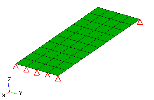
Before you begin, copy the file(s) used in this tutorial to your working directory.
The PSD (power spectral density) for displacement at node 19 is output in the .rand file, and the peak values of PSD and RMS (root mean square) results are output to a .peak file. PSD and RMS stress results are output to a .op2 file and post-processed in HyperView.

random_1
Figure 1.

The frequency analysis setup is already made for this model where the one end of plate is clamped and the loading is applied on the other end (two different sources of the loading, thus two subcases). The loading frequency is defined by the FREQ1 card; from 20 to 1000 Hz with an interval of 20. The same loading frequency is applied on both the subcases.

Launch HyperMesh and Set the OptiStruct User Profile

  1. Launch HyperMesh.
    The User Profile dialog opens.
  2. Select OptiStruct and click OK.
    This loads the user profile. It includes the appropriate template, macro menu, and import reader, paring down the functionality of HyperMesh to what is relevant for generating models for OptiStruct.

Open the Model

  1. Click File > Open > Model.
  2. Select the direct_psd.hm file you saved to your working directory.
  3. Click Open.
    The direct_psd.hm database is loaded into the current HyperMesh session, replacing any existing data.

Set Up the Model

Create TABRND1 Curve

  1. In the Model Browser, right-click and select Create > Curve from the context menu.
  2. For Name, enter tabrnd1.
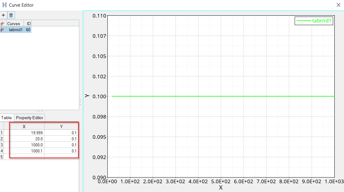
  3. In the Curve Editor window, enter the values shown in Figure 2.


    Figure 2.
  4. Close the Curve Editor window.
  5. In Curves, select tabrnd1.
  6. For Card Image, select TABRND1.

Create RANDPS Load Collector

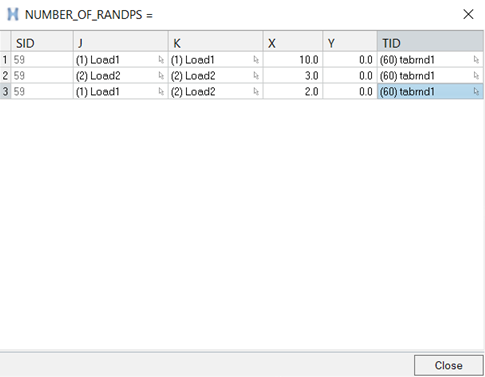
Two PSDF of individual subcases and one coupled PSDF (meaning that those two subcases are correlated) are defined through RANDPS Bulk Data Entry. RANDPS points to the table entity, TABRNDi.
  1. In the Model Browser, right-click and select Create > Load Collector.
  2. For Name, enter randps.
  3. For Card Image, select RANDPS.
  4. For NUMBER_OF_RANDPS=, enter 3 to define three RANDPS entries.
  5. In the NUMBER_OF_RANDPS= dialog, input the parameters.
    The TABRND1 curve is selected for the TID(i) column entries.


    Figure 3.
  6. Click Close.

Add Control Cards and Output Requests

The RANDOM Subcase Information Entry needs to be added to the frequency analysis model and the output commands for RMS and PSD results will be added as well.
  1. From the Analysis page, click control cards.
  2. Go to the GLOBAL_CASE_CONTROL panel.
  3. Check the box in front of RANDOM, double-click the highlighted ID button and select randps.
  4. Return to Control Cards and click GLOBAL_OUTPUT_REQUEST.
  5. Check the box for STRESS to activate the card edit panel.
  6. Select OUTPUT2 as the FORMAT, PSDF under RANDOM, and YES under OPTION.
    RMS and PSDF stress are output to a .op2 file.
  7. Click return to go back to the Control Cards panel.
  8. Select CASE_UNSUPPORTED_CARDS and add the following cards:
    XYPLOT,DISP,PSDF/ 19(T3)
    OptiStruct will output the PSDF for the translational displacement in z direction at node 19.
  9. Click OK, and then click return.

Submit the Job

  1. From the Analysis page, click the OptiStruct panel.

    OS_1000_13_17
    Figure 4. Accessing the OptiStruct Panel
  2. Click save as.
  3. In the Save As dialog, specify location to write the OptiStruct model file and enter direct_psd for filename.
    For OptiStruct input decks, .fem is the recommended extension.
  4. Click Save.
    The input file field displays the filename and location specified in the Save As dialog.
  5. Set the export options toggle to all.
  6. Set the run options toggle to analysis.
  7. Set the memory options toggle to memory default.
  8. Click OptiStruct to launch the OptiStruct job.
If the job is successful, new results files should be in the directory where the direct_psd.fem was written. The direct_psd.out file is a good place to look for error messages that could help debug the input deck if any errors are present.
The default files written to the directory are:
direct_psd.html
HTML report of the analysis, providing a summary of the problem formulation and the analysis results.
direct_psd.out
OptiStruct output file containing specific information on the file setup, the setup of your optimization problem, estimates for the amount of RAM and disk space required for the run, information for each of the optimization iterations, and compute time information. Review this file for warnings and errors.
direct_psd.h3d
HyperView binary results file.
direct_psd.res
HyperMesh binary results file.
direct_psd.stat
Summary, providing CPU information for each step during analysis process.
Also, the following files will be output and which are specific to the random response analysis.
direct_psd.peak
ASCII result file, containing RMS and peak values of PSD.
direct_psd.rand
ASCII result file, containing PSD results.
direct_psd.mvw
HyperView script file. This file will automatically create the plot of PSD over the frequency for the results contained in .rand file.
direct_psd.op2
Binary file containing RMS and PSD results.

View the Results

This step describes how to post-process the RMS and PSD results in HyperView.
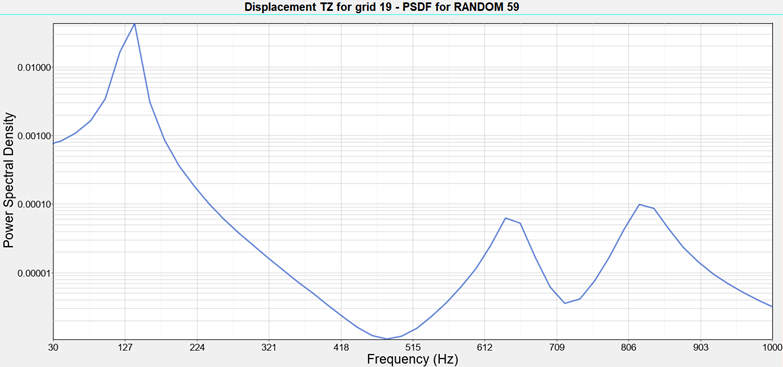
The PSD for displacement at node 19 is output to direct_psd.rand file and the plot of PSD versus frequency can be viewed by loading the direct_psd_rand.mvw file. The RMS and PSD stress results are available in .op2 file. The RMS and the peak values of PSD for displacement at node 19 are output to .peak file, which can be reviewed with any text editor.
  1. Open a HyperView session.
  2. Load the Direct_psd.op2 file.
  3. Go to Contour panel.
  4. In the Load Case and Simulation Selection window, select the random subcase and the frequency = 20.0 Hz as the Simulation.
  5. Select result type PSD STRESS (t), vonMises, and click Apply.
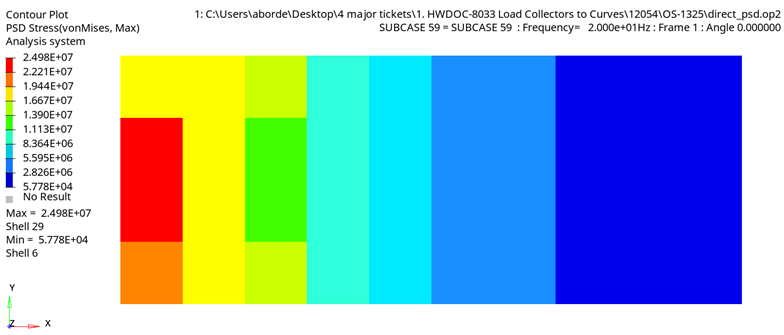
    The PSD vonMises stress contour at frequency 20.0 Hz is displayed as:

    rd2050_contour_plot
    Figure 5.
  6. Change the Simulation to Simulation 1.
  7. Select the result type RMS stress, vonMises, and click Apply.
    The RMS stress contour is displayed.
  8. In the HyperView window, click File > Open > Sessions.
    The Open Session File window opens.
  9. Select the directory where the job was run and select the file direct_psd_rand.mvw.
  10. Click Open.

    random_2
    Figure 6.