Elements
Elements are a fundamental part of any finite element analysis, since they completely represent (to an acceptable approximation), the geometry and variation in displacement based on the deformation of the structure.
Elastic, Damper, and Mass Elements
For such continuum elements, the displacement field over a volume of material which is represented by an element is approximated by corresponding shape functions based on the nodal coordinates. For example, in linear axial elements, the displacement vector is expressed as a linear polynomial whose constants are obtained from the nodal displacements.
Implementation
OptiStruct supports several elements, ranging from 0D, 1D, 2D, to 3D elements. Depending upon the type of analysis, modeling, the level of detail, and the computational time available, any of the available elements, or a combination of them can be selected to achieve the required results.
Zero-dimensional Elements
- CELAS1, CELAS2, CELAS3, and CELAS4 that are used to model elastic springs. The properties for CELAS1 and CELAS3 are defined on PELAS. CELAS2 and CELAS4 define spring properties.
- CDAMP1, CDAMP2, CDAMP3, and CDAMP4 that are used to model scalar dampers. The properties for CDAMP1 and CDAMP3 are defined on PDAMP. CDAMP2 and CDAMP4 define scalar damper properties.
- CMASS1, CMASS2, CMASS3, and CMASS4 that are used to model point masses. The properties for CMASS1 and CMASS3 are defined on PMASS. CMASS2 and CMASS4 define the mass.
- CONM1 and CONM2, which are concentrated mass elements. CONM1 defines a 6x6 mass matrix at a grid point. CONM2 defines mass and inertia properties at a grid point.
- CVISC is used to model viscous dampers. The properties for CVISC are defined on PVISC.
One-dimensional Elements
- Forces and displacements along the axis of the element
- Transverse shear forces (and displacements) in the two lateral directions
- Bending moments (and rotations) in two perpendicular, bending planes
- Torsional moments (and resulting rotations)
- Twisting of the cross-section (or cross-sectional warping)
- CBEAM
- A general beam element that supports all types of action listed above.
- CBAR
- A simple, prismatic beam element that supports all of the above types of actions except cross-sectional warping.
- CBUSH
- A general spring-damper element that supports forces, moments, and displacements along the axis of the element.
- CBUSH1D
- A rod-type spring-damper element.
- CGAP
- A gap element that supports axial and friction forces.
- CGAPG
- A gap element that supports axial and friction forces. It does not have to be placed between grid points. It can also connect surface patches.
- CROD
- A simple, axial bar element that supports only axial forces and torsional moments.
- CWELD
- A simple, axial bar element that supports forces, moments, and torsional moments. It does not have to be placed between grid points. It can also connect surface patches.
- CONROD
- A simple, axial bar element that supports only axial forces and torsional moments. This element does not reference a property definition; the property information is provided with the element definition.
Two-dimensional Shell Elements
Two-dimensional shell elements are used to model thin-shell or thick-shell behavior. Thin-shell behavior can be applied to situations where transverse shear deformation in bending can be ignored, whereas, thick-shell behavior is required in applications where transverse shear appreciably affects model behavior. OptiStruct shell elements have the ability to incorporate in-plane or membrane actions, plane strain, and bending action (including transverse shear characteristics and membrane-bending coupling actions). Reissner-Mindlin shell theory is used to model bending. A plane-strain option is available for pure 2D applications. These properties can be controlled using the PSHELL Bulk Data Entry. For example, the MID# fields on the PSHELL, can be used to define material properties to include bending, transverse shear, membrane-bending coupling, and so on.
The element shapes may be triangular (CTRIA3) or quadrilateral (CQUAD4). Second order triangular (CTRIA6) and quadrilateral (CQUAD8) shell elements are also available.
The first order shell element formulation for CQUAD4 and CTRIA3 has the special characteristic of using six degrees of freedom per grid. Hence, there is stiffness associated to each degree of freedom. In some finite element codes, shell elements do not have a drilling stiffness normal to the mid-plane, which may cause singular stiffness matrix. Then, a user-defined artificial stiffness value is assigned to this degree of freedom to avoid the singularity.
The second order shell elements (CTRIA6 and CQUAD8) have five degrees of freedom per grid. Rotational degrees of freedom without stiffness are removed through SPC.
- Two-dimensional Shell
Element Formulation (Implicit Analysis)
Element formulations indicate the theory used to construct the element, which includes the approximations and improvements applied for an accurate simulation.
The table here is applicable to MAT1, MATS1, and corresponding MAT# entries.Table 1. Summary of Integration Schemes (Implicit Analysis) Linear Analysis Nonlinear Analysis (Contact Nonlinearity only)
Nonlinear Analysis (Geometric Nonlinearity/Plasticity)
Elements In-Plane Through-Thickness Bubble Functions In-Plane Through-Thickness Bubble Functions In-Plane Through-Thickness Bubble Functions CTRIA3 3 point IS Analytical Integration Yes 2 3 point IS Analytical Integration Yes 2 3 point IS 6 point IS 1 Yes 2 CQUAD4 5 point IS Analytical Integration Yes 2 5 point IS Analytical Integration Yes 2 5 point IS 6 point IS 1 Yes 2 CTRIA6 3 point IS Analytical Integration No 3 point IS Analytical Integration No NA NA NA CQUAD8 4 point IS Analytical Integration No 4 point IS Analytical Integration No NA NA NA 1 6-point Gauss-Lobatto quadrature for the through-thickness integration (for models with MATS1).
2 Incompatible modes (bubble function) would introduce additional displacement degree of freedom which are not associated with nodes. Bubble function help add flexibility to the element especially for bending.
3 IS implies Integration Scheme.
- Two-dimensional Shell Element Formulation (Explicit Nonlinear
Analysis)Element formulations indicate the theory used to construct the element, which includes the approximations and improvements applied for an accurate simulation. For explicit analysis, the integration scheme can be changed using ISOPE field on PSOLID, PLSOLID, or PSHELL entries, or via PARAM,EXPISOP. The settings on the ISOPE field will overwrite the settings on PARAM,EXPISOP.
Table 2. Summary of Integration Schemes (Explicit Nonlinear Analysis) Belytschko-Tsay (ISOPE=1)
Belytschko-Wong-Chiang with drill projection (ISOPE=2)
Belytschko-Wong-Chiang with full projection (ISOPE=3)
C0 Triangular Shell (ISOPE=4)
Elements In-Plane Through-Thickness In-Plane Through-Thickness In-Plane Through-Thickness In-Plane Through-Thickness CTRIA3 NA NA NA NA NA NA 1 point IS 3 point IS 1 CQUAD4 1 point IS 3 point IS 1 1 point IS 3 point IS 1 1 point IS 3 point IS 1 NA NA 1 Through the thickness direction, the default number of integration points for Explicit analysis is 3 points. This can be controlled using the NIP field on PSHELL entry. The value of NIP can vary from 1 to 10. (a) To mimic membrane behavior, NIP can be set to 1 and/or MID2 can be left blank. (b) For elastic material, NIP can be set to 2. (c) For nonlinear material, NIP should be set to a minimum of 3.
2 IS implies Integration Scheme
- Two-dimensional
Axisymmetric Solid Elements (Implicit Analysis)Two-dimensional Axisymmetric solid elements CTAXI, CTRIAX6, and CQAXI are available. CTAXI and CTRIAX6 are triangular, and CQAXI is a quadrilateral axisymmetric element. The materials for these elements can be defined by MAT1, MAT3, MATS1, and MATHE entries. The properties for these elements are defined by PAXI entry.
Table 3. Summary of Integration (Implicit Analysis) Linear Analysis Nonlinear Analysis (MAT# or MAT# with MATS1)
Nonlinear Analysis (MATHE)
Elements Regular Elements 1 Regular Elements 1 Regular Elements 1 CQAXI (1st order)
4 point IS 4 point IS 5 point IS CTAXI (1st order)
3 point IS 3 point IS 3 point IS CTRIAX6 (1st order)
3 point IS 3 point IS 3 point IS CQAXI (2nd order)
9 point IS 9 point IS 9 point IS CTAXI (2nd order)
7 point IS 7 point IS 3 point IS CTRIAX6 (2nd order)
7 point IS 7 point IS 3 point IS 1 Contact Friendly elements are not supported for 2D axisymmetric solid elements.
2 IS implies Integration Scheme
- Two-dimensional
Plane-Strain Elements (Implicit Analysis)Two-dimensional plane-strain elements CQPSTN and CTPSTN are available. CTPSTN is triangular, and CQPSTN is a quadrilateral plane-strain element. The materials for these elements can be defined by MAT1, MAT3, and MATHE entries. The properties for these elements are defined by PPLANE entry.
Table 4. Summary of Integration (Implicit Analysis) Linear Analysis Nonlinear Analysis (MAT#)
Nonlinear Analysis (MATHE)
Elements Regular Elements 1 Regular Elements 1 Regular Elements 1 CQPSTN (1st order)
4 point IS 4 point IS 5 point IS CTPSTN (1st order)
3 point IS 3 point IS 3 point IS CQPSTN (2nd order)
9 point IS 9 point IS 9 point IS CTPSTN (2nd order)
7 point IS 7 point IS 3 point IS 1 Contact Friendly elements are not supported for two-dimensional plane-strain elements.
2 IS implies Integration Scheme
Three-dimensional Solid Elements
- Three-dimensional Solid Element Formulation (Implicit Analysis)
Element formulations indicate the theory used to construct the element, which includes the approximations and improvements applied for an accurate simulation. The number of integration points mentioned here are the generic defaults. Depending on the solution and model parameters, a different number of integration points may be used. For example, Hyperelastic elements or integration points on surfaces of solids.
Table 5. Summary of Integration Schemes (Implicit Analysis) Linear Analysis Nonlinear Analysis MAT# or MAT# with MATS1, MATVE, MATVP MATHE Elements Regular Elements Contact-Friendly Elements Regular Elements (ISOP=FULL) Contact-Friendly Elements (ISOP=FULL) Regular Elements (ISOP=MODPLAST) Regular Elements (ISOP=REDPLAST) Regular Elements (ISOP=INT0) Regular Elements CTETRA (1st order)
1 point IS NA 1 point IS NA 1 point IS 1 point IS 1 point IS 4 point IS CHEXA (1st order)
8 point IS NA 8 point IS NA 8 point IS 8 point IS 9 point IS 8 point IS CTETRA (2nd order)
4 point IS 5 point IS 5 point IS 5 point IS 5 point IS 4 point IS 9 point IS 4 point IS CHEXA (2nd order)
27 point IS 27 point IS 27 point IS 27 point IS 14 point IS 9 point IS 27 point IS 8 point IS CPENTA (1st order)
6 point IS NA 6 point IS NA 6 point IS 6 point IS 12 point IS 6 point IS CPENTA (2nd order)
21 point IS 21 point IS 21 point IS 21 point IS 21 point IS 12 point IS 28 point IS 6 point IS CPYRA (1st order)
8 point IS NA 8 point IS NA 8 point IS 8 point IS 9 point IS NA CPYRA (2st order)
27 point IS 27 point IS 27 point IS 14 point IS 27 point IS 9 point IS 27 point IS NA 1 IS implies Integration Scheme
Table 6. Summary of Integration Schemes for Gasket Elements (Implicit Analysis) Linear Analysis Nonlinear Analysis Elements Regular Elements Contact Friendly Elements Regular Elements Contact Friendly Elements CGASK8 4 point IS NA 4 point IS NA CGASK6 3 point IS NA 3 point IS NA CGASK16 9 point IS 25 point IS 9 point IS 25 point IS CGASK12 7 point IS 19 point IS 7 point IS 19 point IS 1 The integration points are located on the mid-plane of the 3D gasket elements.
2 IS implies Integration Scheme
- Three-dimensional
Solid Element Formulation (Explicit Nonlinear Analysis)Element formulations indicate the theory used to construct the element, which includes the approximations and improvements applied for an accurate simulation. Note that the number of integration points mentioned here are the generic defaults. Depending on the solution and model parameters, a different number of integration points may be used. For example, Hyperelastic elements or integration points on surfaces of solids. For explicit analysis, the integration scheme can be changed using the ISOPE field on PSOLID, PLSOLID, or PSHELL entries, or via PARAM,EXPISOP. The settings on the ISOPE field will overwrite the settings on PARAM,EXPISOP.
Table 7. Summary of Integration Schemes (Explicit Nonlinear Analysis) Elements Regular Elements (ISOPE=URI) Regular Elements (ISOPE=AURI) Regular Elements (ISOPE=SRI) Regular Elements (Full Integration)
CHEX (1st order)
Uniform Reduced Integration 1-point IS
Average Reduced Uniform Integration B matrix is volume-averaged over the element
Selective Reduced Integration Full IS for deviatoric term and 1-point IS for bulk term
NA CTETRA (2nd order)
NA NA NA 5 point IS CPENTA (1st order)
NA NA Selective Reduced Integration Full IS for deviatoric term and 1-point IS for bulk term
NA CTETRA (1st order)
NA NA NA 1 point IS 1 IS implies Integration Scheme
Interface Elements
Interface elements are elements which are specialized for a particular purpose of simulating behavior at the interfaces between structures or on the surface of the structural elements interacting with the environment (for example, CHBDYE - thermal boundary surface elements, CIFPEN/CIFHEX - cohesive elements, and so on).
| Elements | Gaussian IS Default: INT=0 (On PCOHE) |
Newton-Cotes IS =1 (On PCOHE) |
|---|---|---|
| CIFPEN (1st order) |
3 point IS | 3 point IS |
| CIFHEX (1st order) |
4 point IS | 4 point IS |
| CIFPEN
(1st order) |
7 point IS | 6 point IS |
| CIFHEX
(2nd order) |
9 point IS | 8 point IS |
1 The number of integration points listed is for each surface of the cohesive elements. Each Cohesive element has two surfaces.
2 IS implies Integration Scheme
Offset for One-dimensional and Two-dimensional Elements
Some one-dimensional and two-dimensional elements can use offset to “shift” the element stiffness relative to the location determined by the element’s nodes. For example, shell elements can be offset from the plane defined by element nodes by means of ZOFFS. In this case, all other information, such as material matrices or fiber locations for the calculation of stresses, are given relative to the offset reference plane. Similarly, the results, such as shell element forces, are output on the offset reference plane.
Offset is applied to all element matrices (stiffness, mass, and geometric stiffness), and to respective element loads (such as gravity). Hence, in principle, offset can be used in all types of analysis and optimization.

Figure 1.
Furthermore, in a fully nonlinear approach, additional instability points may be present on the limit load path.
Comments
- Through-Thickness direction, the default number of integration
points for Explicit analysis is 3 points. This can be controlled using the
NIP field on PSHELL entry. The
value of NIP can vary from 1 to 10.
- To mimic membrane behavior, NIP can be set to 1
- For elastic material, NIP can be set to 2
- For nonlinear material, NIP should be set to a minimum of 3
Non-structural Mass
Non-structural mass may be specified in two different ways.
- Many property definitions (PSHELL, PCOMP, PBAR, PBARL, PBEAM, PBEAML, PROD, CONROD, PSHEAR, and PTUBE), have an NSM data field that allows a value
of non-structural mass per unit area or non-structural mass per unit length to be defined.
When non-structural mass is defined in this way, it is considered in all analyses.
- Non-structural mass may be defined via a number of non-structural mass Bulk Data Entries
(NSM, NSM1, NSML, NSML1, and NSMADD) for a list of elements or properties.
In the case of a list of properties, non-structural mass is applied to the elements
referencing the properties in the list.
These non-structural mass definitions must be selected for use in an analysis through the NSM Subcase Information Entry.
The NSM Subcase Entry is currently subcase-dependent only for Linear Static and Nonlinear Static Analysis. For all other solution sequences, the NSM Subcase Entry should be defined globally above the first SUBCASE statement. If the NSM Subcase Entry is specified within any subcase which is not linear static or nonlinear static, then the run will be terminated with an error.- Input non-structural mass per unit area/length/volume
(NSM/NSM1)
The NSM Bulk Data Entry and its alternate form NSM1 allow you to define a value of non-structural mass per unit area, non-structural mass per unit length, or non-structural mass per unit volume to be applied to a selected list of elements
The NSM field on various property entries listed above also inputs mass per unit area/length/volume directly.
- Input lumped non-structural mass
(NSML/NSML1)The NSML Bulk Data Entry and its alternate form NSML1 allow you to allocate and smear a lumped non-structural mass value to be evenly distributed over a list of elements.
- Default Distribution (DTYPE=blank on
NSML/NSML1)The non-structural mass value per unit area, per unit length, or per unit volume to be applied to the elements is:
(1) (2) (3) For the default case when DTYPE is blank, referencing a mixture of different element or property types is not supported.
- Distribution based on Mass/Volume
(DTYPE=MASS/VOLUME on
NSML/NSML1)The non-structural mass value per unit mass or volume to be applied to the elements is:
(4) (5)
- Default Distribution (DTYPE=blank on
NSML/NSML1)
Where,- Number of elements in the set
- Value of the lumped mass
- Length of element
- Area of element
- Volume of element
- Mass of element
An important difference between the default distribution (DTYPE=blank) and DTYPE=MASS/VOLUME, is that a mixture of multiple element types (1D, 2D, and 3D elements) can be defined on a single NSML/NSML1 entry when TYPE field is set to ELEMENT/ELSET (mixture of elements) or MIXED (mixture of properties).
- Input non-structural mass per unit area/length/volume
(NSM/NSM1)
The NSMADD Bulk Data Entry allows you to form combinations of NSM, NSM1, NSML, and NSML1.
An element can have more than one non-structural mass value specified for it. The actual non-structural mass value will be the sum of all of the individual non-structural mass values.
Virtual Fluid Mass
Virtual Fluid Mass mimics the mass effect of an incompressible inviscid fluid in contact with a structure. There is no mesh needed for the fluid domain. The Virtual Fluid Mass represents the full coupling between acceleration and pressure at the fluid-structure interface.
A dense mass matrix is generated among damp grids at the fluid-structure interface. This simulation is applicable to automobile containers, such as a fuel tank, which hold non-pressurized fluids.
Assumptions
- The fluid is inviscid and incompressible. The fluid flow is a potential flow.
- Because the fluid is nearly incompressible, the structural modes are below the compressible fluid modes.
- There is no gravity effect or sloshing effect.
- There is no acoustic effect involved. The modes from the structural side do not couple with the modes of the nearly incompressible fluid modes.
- Fully enclosed wet surface without any open surface is currently not supported.
MFLUID Interface
- PARAM,VMOPT
If PARAM,VMOPT,1 is used (default), the virtual mass is included in the regular mass matrix and it can be applied to both direct and modal dynamic subcases. Because the virtual mass matrix is dense for the damp grids, the computational time increases significantly.
However, you have the option to use PARAM,VMOPT,2; although, PARAM,VMOPT,2 can only be applied to modal dynamic subcases. In this case, the virtual mass is added after the eigen solution, and the computational time is not increased significantly. When PARAM,VMOPT,2 is used, the dry modes are computed without adding virtual mass in the computation. Then the modes are modified based on the virtual mass matrix.
To generate accurate wet modes results with PARAM,VMOPT,2, it is recommended to request 2 to 4 times (or even higher, depending on the density of fluid) the number of dry modes than the desired number of wet modes. If the density of fluid is larger, the number of dry modes required could be larger accordingly in order to maintain the accuracy of wet modes that are based on dry modes.
- PARAM,VMMASS
PARAM,VMMASS,YES can be used in conjunction with PARAM,VMOPT,1 to include MFLUID mass to the Grid Point Weight Generator output in the .out file.
Theory
An additional area integration is done to convert pressure into force.
Using the force and acceleration, the effective mass matrix can be calculated.
Arbitrary Beam Section Definition
In addition to using predefined beam cross-sections selected by the TYPE field on the PBARL and PBEAML Bulk Data Entries, defining arbitrary beam cross-sections. This is referred to here as section definitions. To define an Arbitrary Beam Section, HYPRBEAM should be entered into the GROUP field on the PBARL and PBEAML Bulk Data Entries. Also, the ND field should specify the number of dimensions input during the definition of the arbitrary beam section in the DIMi fields of the PBARL and PBEAML Bulk Data Entries.
Section definitions are contained within the Bulk Data section of the input file. A section definition begins with the statement BEGIN and ends with the statement END. Section definitions are referenced from a PBARL or PBEAML definition through the NAME field. The NAME entered on the PBARL or PBEAML definition must match the NAME following the BEGIN statement.
The section is defined by a 2D finite element mesh. The finite element mesh is composed of nodes (specified by GRIDS entries), which are connected by 2-node, 3-node, 4-node, 6-node or 8-node elements (specified by CSEC2, CSEC3, CSEC4, CSEC6, or CSEC8 entries, respectively). These elements reference PSEC entries; these provide a material reference for all elements and thickness information for the 2-noded CSEC2 elements.
Example: Simple Thin-walled Section Definition Named SQUARE
$
BEGIN,HYPRBEAM,SQUARE
$
GRIDS,1,0.0,0.0
GRIDS,2,1.0,0.0
GRIDS,3,1.0,1.0
GRIDS,4,0.0,1.0
$
CSEC2,10,100,1,2
CSEC2,20,100,2,3
CSEC2,30,100,3,4
CSEC2,40,100,4,1
$
PSEC,100,1000,0.1
$
END,HYPRBEAM
$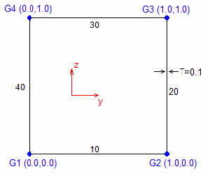
Figure 2.
Example: Solid Section Definition Named CUTOUT
$
BEGIN,HYPRBEAM,CUTOUT
$
GRIDS,1,0.0,0.0
GRIDS,2,0.05,0.0
...
...
GRIDS,895,0.35,1.18
GRIDS,896,0.38,1.19
$
CSEC3,806,100,887,873,872
CSEC3,809,100,868,820,885
CSEC3,812,100,813,803,817
$
CSEC4,1,100,147,148,149,157
CSEC4,2,100,157,149,150,158
...
...
CSEC4,813,100,648,712,895,896
CSEC4,814,100,647,646,896,895
$
PSEC,100,1000
$
END,HYPRBEAM
$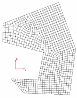
Figure 3.
Rigid Elements and Multi-Point Constraints
Rigid elements and multi-point constraints are used to constrain one or more degrees of freedom to be equal to linear combinations of the values of other degrees of freedom.
Rigid elements are equations generated internally. You provide the connection data only. Rigid elements function as rigid bodies; therefore they are also known as rigid bodies or constraint elements. Internally, they are treated the same way as multi-point constraints.
The RROD element can be used to model a pin-ended rod which is rigid in extension. One equation of constraint will be generated for this element. The RBAR element can be used to model a rigid bar with six degrees of freedom at each end. Anywhere from one to six (depending on your input) equations of constraint will be generated for this element.
The RBE1 and RBE2 elements are rigid bodies connected to an arbitrary number of grid points. The number of equations of constraint generated is equal to or greater than one, depending on the dependent degrees of freedom selected by you. For the RBE1 element, the independent degrees of freedom are six components of motion that must be jointly capable of representing any general rigid body motion of the element; whereas for the RBE2 element, the independent degrees of freedom are the six components of motion at a single grid point.
The RBE3 element provides for specification from one to six equations of constraint developed from the relation that the motion at a "reference grid point" is the least square weighted average of the motion at other grid points. This element is generally used to "beam" loads and masses from a reference point to a set of grid points. Multi-point constraints are equations in which you explicitly provide the coefficients of the equations. Each multi-point constraint is described by a single equation that specifies a linear relationship for two or more degrees of freedom. Multiple sets of multi-point constraints can be provided in the Bulk Data section. In the Subcase Information section, the multi-point constraints are assigned to the specific load case using the MPC statement.
The Bulk Data Entry MPC is the statement for defining multi-point constraints. The first coordinate mentioned on the card is taken as the dependent degree of freedom (that is, the degree of freedom that is removed from the equations of motion). Dependent degrees of freedom may appear as independent terms in other equations of the set; however, they may appear as dependent terms in only a single equation.
- To enforce zero motion in directions other than those corresponding to components of the global coordinate system. In this case, the multi-point constraint will involve only the degrees of freedom at a single grid point. The constraint equation relates the displacement in the direction of zero motion to the displacement components in the global system at the grid point.
- To describe rigid elements and mechanisms such as levers, pulleys, and gear trains. In this application, the degrees of freedom associated with the rigid element that are in excess of those needed to describe rigid body motion are eliminated with multi-point constraint equations. Treatment of very stiff members as being rigid elements eliminates the ill-conditioning associated with their treatment as ordinary elastic elements.
- To be used with scalar elements to generate non-standard structural elements and other special effects.
- A dependent degree of freedom cannot be in the SPC.
- A dependent degree of freedom in any rigid element or multi-point constraint cannot be defined as a dependent degree of freedom in any other rigid element or multi-point constraint.
JOINTG (Connectors)
The various joints identified by the JTYPE field require certain corresponding coordinate system rules.
Universal Joint
A Universal Joint is a joint which allows rotary motion transmission in multiple shafts which are at an angle to each other (for example, in a powertrain drive shaft). The joint works by allowing free rotation along two mutually perpendicular degrees of freedom of the two grid points associated with the joint. The remaining rotational degrees of freedom are automatically constrained. The translational degrees of freedom can be constrained by defining an additional Ball joint.
- JTYPE should be set to UNIVERSA.
- The X-axis of the coordinate system (CID1) of Grid Point 1 should be mutually perpendicular to the Z-axis of coordinate system (CID2) of Grid Point 2.
- The Y-axes of coordinate systems 1 and 2 should be along the corresponding shaft axes. Additionally, they should point in the same direction (should not point opposite to one another).
- The translational degrees of freedom can be constrained by defining an additional Ball joint.

Figure 4.
Revolute Joint
A Revolute Joint is a joint which allows single axis rotation functions (for example, in a door hinge). The joint works by allowing free rotation (or enforced displacement via MOTNJG) about one degree of freedom of the two grid points associated with the joint (the two selected degrees of freedom should be the same). The remaining rotational degrees of freedom are automatically constrained. The translational degrees of freedom can be constrained by defining an additional Ball joint.
- JTYPE should be set to REVOLUTE.
- The X-axis of the coordinate system (CID1) of Grid Point 1 should be parallel (and in the same direction) to the X-axis of coordinate system (CID2) of Grid Point 2. The MOTNJG Subcase Information and Bulk Data Entries can be used to define the value of rotation (dof=4) about the X-axis.
- The other axes of the coordinate system may point in any direction.
- The translational degrees of freedom can be constrained by defining an additional Ball joint.

Figure 5.
Ball Joint
A Ball Joint is a joint which allows free rotation in all three directions and translations are constrained in all three directions (for example, in automobile steering and suspension systems). The joint works by allowing free rotation about all three degrees of freedom of the two grid points associated with the joint. The remaining translational degrees of freedom are constrained. For BALL joint, there is no relative translation between the two degrees of freedom in the basic system. Local systems should not be defined for the BALL joint and will not be used if specified.
- JTYPE should be set to BALL.
- Only the grid points GID1 and GID2 should be specified. The coordinate systems are not required.
- The grid points GID1 and GID2 should be
coincident to simulate physical joints. If they are not, the specified joint may deviate
from expected behavior.

Figure 6.
Axial Joint
An Axial Joint is a joint which allows connection between two grid points by enforcing relative displacement along the line joining them. The relative displacement is enforced only along the line connecting the two grid points, and other degrees of freedom are not constrained by this joint.
- JTYPE should be set to AXIAL.
- Only the grid points GID1 and GID2 should be specified. The coordinate systems are not required and will be ignored if specified.
- The MOTNJG Bulk Data Entry should be used to identify the value of the enforced relative displacement via the VALUE field (). The MOTNJG Subcase Information Entry can then be used to identify the corresponding MOTNJG Bulk Data Entries.
- To hold the value of the relative displacement from the previous subcase in the subsequent nonlinear subcase (via CNTNLSUB), the VALUE field can be set to FIXED on the MOTNJG Bulk Data Entry. Alternatively, a different value of relative motion can be specified for the continuing subcase.

Figure 7.
Cartesian Joint
A Cartesian Joint allows connection between two grid points by enforcing relative displacement along three directions (1,2,3) of a local Cartesian coordinate system CID1 defined on GID1. The other degrees of freedom are not constrained by this joint.
- JTYPE should be set to CARTES.
- The grid points GID1 and GID2 should be specified. The coordinate system CID1 on GID1 is required. CID2 is not required and will be ignored if specified.
- The MOTNJG Bulk Data Entry should be used to identify the value of the enforced relative displacement via the VALUE fields corresponding to the 1, 2, and 3 degrees of freedom. The MOTNJG Subcase Information Entry can then be used to identify the corresponding MOTNJG Bulk Data Entries.
- To hold the value of the relative displacement from the previous subcase in the subsequent nonlinear subcase (via CNTNLSUB), the VALUE field can be set to FIXED on the MOTNJG Bulk Data Entry. Alternatively, a different value of relative motion can be specified for the continuing subcase.
Cardan Joint
A Cardan Joint allows connection between two grid points by enforcing relative rotation along three directions (4,5,6). Three successive rotations are performed based on the Cardan angles that correspond to the local coordinate system directions at GID1 and GID2. The other degrees of freedom are not constrained by this joint.
- JTYPE should be set to CARDAN.
- The grid points GID1 and GID2 should be specified. The coordinate system CID1 is required. CID2 is not required and will be ignored if specified.
- The MOTNJG Bulk Data Entry should be used to identify the value of the Cardan angles via the VALUE fields corresponding to the 4, 5, and 6 degrees of freedom. The MOTNJG Subcase Information Entry can then be used to identify the corresponding MOTNJG Bulk Data Entries.
- To hold the value of the relative displacement from the previous subcase in the subsequent nonlinear subcase (via CNTNLSUB), the VALUE field can be set to FIXED on the MOTNJG Bulk Data Entry. Alternatively, a different value of relative motion can be specified for the continuing subcase.
In-Plane Joint
An in-plane joint allows connection between two grid points by enforcing zero relative displacement along direction 1 of a local Cartesian coordinate system CID1 defined on GID1. Additionally, enforced relative displacement is applied in the 2 and 3 directions of CID1. The other degrees of freedom are not constrained by this joint.
- JTYPE should be set to INPLANE.
- The grid points GID1 and GID2 should be specified. The coordinate system CID1 on GID1 is required. CID2 is not required and will be ignored if specified.
- The MOTNJG Bulk Data Entry should be used to identify the value of the enforced relative displacement via the VALUE fields corresponding to the 2, and 3 degrees of freedom. The MOTNJG Subcase Information Entry can then be used to identify the corresponding MOTNJG Bulk Data Entries.
- To hold the value of the relative displacement from the previous subcase in the subsequent nonlinear subcase (via CNTNLSUB), the VALUE field can be set to FIXED on the MOTNJG Bulk Data Entry. Alternatively, a different value of relative motion can be specified for the continuing subcase.
In-Line Joint
An in-line joint allows connection between two grid points by enforcing zero relative displacement along directions 2 and 3 of a local Cartesian coordinate system CID1 defined on GID1. Additionally, enforced relative displacement is applied in the 1 direction of CID1. The other degrees of freedom are not constrained by this joint.
- JTYPE should be set to INLINE.
- The grid points GID1 and GID2 should be specified. The coordinate system CID1 on GID1 is required. CID2 is not required and will be ignored if specified.
- The MOTNJG Bulk Data Entry should be used to identify the value of the enforced relative displacement via the VALUE field corresponding to the 1 degree of freedom. The MOTNJG Subcase Information Entry can then be used to identify the corresponding MOTNJG Bulk Data Entries.
- To hold the value of the relative displacement from the previous subcase in the subsequent nonlinear subcase (via CNTNLSUB), the VALUE field can be set to FIXED on the MOTNJG Bulk Data Entry. Alternatively, a different value of relative motion can be specified for the continuing subcase.
Orient Joint
An Orient joint allows connection between two grid points by enforcing zero relative rotations along directions 4, 5, and 6 of two local Cartesian coordinate systems CID1 and CID2. The other degrees of freedom are not constrained by this joint.
- JTYPE should be set to ORIENT.
- The grid points GID1 and GID2 should be specified.
- The coordinate systems CID1 and CID2 are required.
Hinge Joint
A Hinge joint allows connection between two grid points by enforcing zero relative translations along directions 1, 2, and 3 of two local Cartesian coordinate systems CID1 and CID2. Additionally, the relative rotations in 5 and 6 are also constrained. Only degree of freedom 4 is not constrained by this joint. The joint works by allowing free rotation in degree of freedom 4 of the two grid points associated with the joint (the two X axes of both CID1 and CID2 should match for this joint).
- JTYPE should be set to HINGE.
- The grid points GID1 and GID2 should be specified. The coordinate systems CID1 and CID2 are required.
- The X-axes of both CID1 and CID2 should match.
- The Hinge joint is equivalent to a combination of Revolute joint and Rigid Pin joint.
Rigid Pin Joint
A Rigid Pin joint allows connection between two grid points by enforcing zero relative translations along directions 1, 2, and 3 of a local Cartesian coordinate system CID1 defined on grid GID1. The joint works by allowing free rotation in degrees of freedom 4, 5 and 6 of the two grid points associated with the joint. For RPIN joint, there is no relative translation between the grids in the local system defined on CID1 (this is where RPIN differs from BALL joint). Note that for any local system defined on a grid for the joints, the local systems move/rotate along with the grids on which they are defined. Therefore, even though from the perspective of the basic system, there may seem to be relative translation between the grids in RPIN joint, there will not be any relative translation between the grids in the local CID1 which moves/rotates with grid GID1.
- JTYPE should be set to RPIN.
- The grid points GID1 and GID2 should be specified.
- The coordinate systems CID1 is required and CID2 should not be specified. CID2 will be ignored if defined.
Rigid Link Joint
- JTYPE should be set to RLINK.
- The grid points GID1 and GID2 should be specified.
- The coordinate systems CID1 and CID2 should not be specified and will be ignored if defined.
Rigid Beam Joint
- JTYPE should be set to RBEAM.
- The grid points GID1 and GID2 should be specified.
- By default, CID1 and CID2 are defined as the
basic coordinate system and the results are output in the basic coordinate system.
If a local coordinate system is assigned to these fields, the results are output in the local coordinate system.
- The Rigid Beam joint is equivalent to a combination of Rigid Pin joint and Orient joint.
Universal Connection with Rigid Pin Joint
- JTYPE should be set to UJOINT.
- The X-axis of the coordinate system (CID1) of Grid Point 1 should be mutually perpendicular to the Z-axis of coordinate system (CID2) of Grid Point 2.
- The Y-axes of coordinate systems 1 and 2 should be along the corresponding shaft axes. Additionally, they should point in the same direction (should not point opposite to one another).
- The grid points GID1 and GID2 should be specified.
- The coordinate systems CID1 and CID2 should also be specified and follow the setup mentioned in points 2 and 3 above.
The UJOINT joint is equivalent to a combination of Rigid Pin joint and Universal joint.
Cylindrical Joint
- JTYPE should be set to CYLINDRI.
- The grid points GID1 and GID2 should be specified.
- The coordinate systems CID1 and CID2 should be specified and the direction 1 of both systems should match
The Cylindrical joint is equivalent to a combination of In-Line joint and Revolute joint.
Translator Joint
- JTYPE should be set to TRANSLAT.
- The grid points GID1 and GID2 should be specified.
- The coordinate systems CID1 and CID2 should be specified.
The Translator joint is equivalent to a combination of In-Line joint and Orient joint.
Combination Joints
Axial and Orient Joint
- JTYPE should be set to AXIAORIE.
- The grid points GID1 and GID2 should be specified. The coordinate systems CID1 and CID2 should be specified.
Inline and Cardan Joint
- JTYPE should be set to INLICARD.
- The grid points GID1 and GID2 should be specified. The coordinate systems CID1 and CID2 should be specified.
Rigid Link and Orient Joint
- JTYPE should be set to RLINORIE.
- The grid points GID1 and GID2 should be specified. The coordinate systems CID1 and CID2 should be specified.
Define Local Coordinate Systems for JOINTG
Local coordinate systems (via CID1 and CID2) are important to define the interpretation of joint loading (LOADJG), joint motion (MOTNJG), and for STOP and LOCK options (PJOINTG).
Interpretation of Joint Characteristics
- Order of joint grids, GID1 and
GID2.The order of GID1 and GID2 influences the calculation of relative displacement between the two grids. Typically for a particular degree of freedom, the relative displacement is calculated as:
(9) Where, and are displacements of GID1 and GID2 in a particular degree of freedom.
- Local Coordinate System(s) CID1 and
CID2 at GID1 and
GID2, respectively.
Direction of the degree of freedom of interest identified via CID1 or CID2 influences the interpretation of length, motion, STOP, LOCK options, and output.
- Nature of applied loading, motion, or value of
STOP/LOCK.
For instance, the effect of compressive loading (negative LOADJG) on the joint is opposite to that of tensile loading (positive LOADJG).
The following sections investigate in detail, the interpretation of individual joint characteristics. Simple examples with corresponding JOINTG are used to illustrate the concepts, as well.
Joint Loading (LOADJG)
Loading on a joint can be applied using LOADJG entry or via other external loads. Here you will study the behavior of loading using LOADJG.
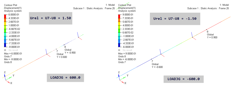
Figure 8.
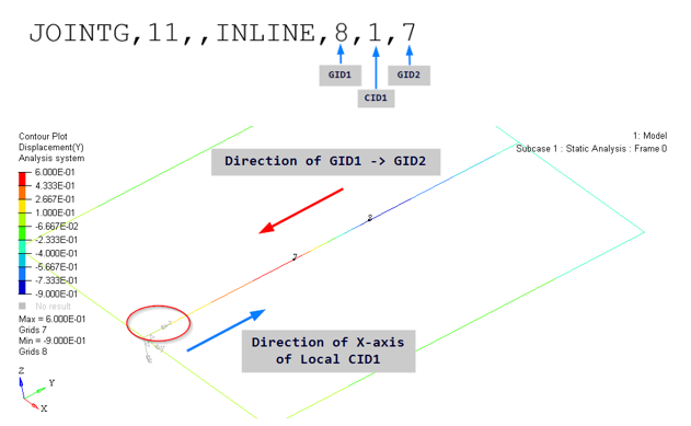
Figure 9.
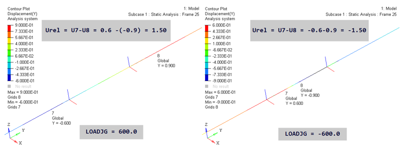
Figure 10.
The key here is the calculation of U7 and U8. In the LOADJG=600.0 image above, U7 in basic Y is -0.6. Since Local X was flipped, it points opposite to basic Y. Therefore, U7 in local X is +0.6. Similarly, U8 in basic Y is 0.9 and in local X it is -0.9. Therefore, U7-U8 in local X is 1.5. The value of U7 and U8 for LOADJG=-600.0 case can also be inferred similarly.
Figure 11.
Enforced Joint Motion (MOTNJG)
Enforced Motion on a joint can be applied using MOTNJG entry or via other external SPCD entries. In this section, you will study the behavior of loading using MOTNJG.
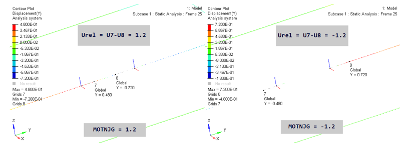
Figure 12.
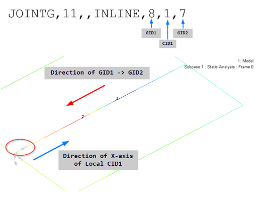
Figure 13.
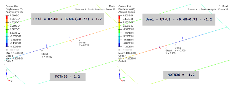
Figure 14.
The key here is the calculation of U7 and U8. In the MOTNJG=1.2 image above, U7 in basic Y is -0.48. Since Local X was flipped, it points opposite to basic Y. Therefore, U7 in local X is +0.48. Similarly, U8 in basic Y is 0.72 and in local X it is -0.72. Therefore, U7-U8 in local X is 1.2. The value of U7 and U8 for MOTNJG=-1.2 case can also be inferred similarly.
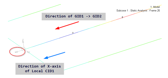
Figure 15.
STOP and LOCK (PJOINTG)
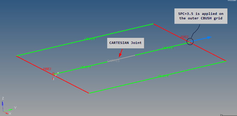
Figure 16.
- When local X is aligned with GID1 → GID2, the length is positive and to apply an absolute upper limit of 2.2, the upper bound field of LOCK should be set to 2.2.
- When local X is opposite to GID1 → GID2, the length is negative and to apply an absolute upper limit of 2.2, the lower bound field of LOCK should be set to -2.2.
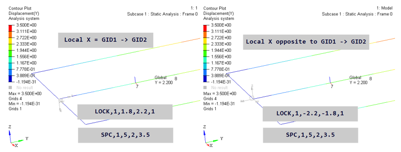
Figure 17.
Based on the CARTESIAN joint example in Figure 16, you can infer the process of applying similar constraints on the length of other joints of other degrees of freedom of interest, depending on the interplay of GID1 → GID2 direction and the local axis direction of the degree of freedom of interest.
Composite Laminates
Shells and solid elements can be made of composites in which several layers of different materials (plies) are bonded together to form a cohesive structure.

Figure 18. Four-layer Composite Shell with Ply Angle
Classical lamination theory is used to calculate effective stiffness and mass density of the composite shell. This is done automatically within the code using the properties of individual plies. The homogenized shell or solid properties are then used in the analysis.
After the analysis, the stresses and strains in the individual layers and between the layers can be calculated from the overall shell stresses and strains. These results may then be used to assess the failure indices of individual plies and of the bonding matrix.
Analysis of Composite Shells (PCOMP, PCOMPG, PCOMPP)
Analysis of composite shells is similar to the solution of standard shell elements. The primary difference is the use of the PCOMP, PCOMPP or PCOMPG property card, instead of PSHELL, to specify shell element properties.
From the ply information specified on the corresponding PCOMP, PCOMPG entries or from the PLY entries (in case of PCOMPP), OptiStruct automatically calculates the effective properties of the shell element.
After the analysis, the available results include shell-type stresses as well as stresses, strains, and failure indices for individual plies and their bonding. These results are controlled by the results flags on the PCOMP or PCOMPG entry and the typical I/O control cards, including CSTRESS, CSTRAIN, and CFAILURE entries.
- Differences between PCOMP and
PCOMPG
PCOMP and PCOMPG define the composite lay-up in two different ways.
PCOMP defines the structure and properties of a composite lay-up, which is then assigned to an element. The plies are only defined for a particular property and there is no relationship of plies that reach across several properties.
PCOMPG defines the structure and properties of a composite lay-up allowing for global ply identification which is then assigned to an element. The plies of different PCOMPG definitions can have a relationship because of the use of global ply IDs.
- PCOMPP
PCOMPP allows ply-based modeling using PLY and STACK entries to define plies. The element sets to which plies are assigned are identified on the PLY entries via the ESID# fields. The stacking information and stacking sequence are defined via the STACK entries. Optionally, substacks and interface definitions are also possible using the STACK entries.
- The most typical material type used for composite plies is MAT8, which is planar orthotropic material. The use of isotropic MAT1 or general anisotropic MAT2 for ply properties is also supported.
- While it is possible to specify ply angles relative to the element coordinate system, the results become strongly dependent upon the node numbering in individual elements. Thus, it is advisable to specify a material coordinate system for composite elements and specify ply angles relative to this system.
- Depending on the specific lay-up structure, the composite may be offset from the reference plane of the shell element, i.e. have more material below than above the reference plane (or vice versa).
- Stress results for composites include both shell-type stresses and individual ply stresses. Importantly, shell-type stresses are calculated using homogenized properties and thus only represent the overall stress-state in the shell. To assess the actual stress-state in the composite, individual ply results need to be examined.
Analysis of Continuum Shells (PCOMPLS)
Continuum Shells can be effective in dealing with a three-dimensional stress state and/or if the laminate thickness is high enough that the classical shell theory limitations are met.
Analysis of Continuum Shells involves using the PCOMPLS entry to assign ply information to solid elements. This is currently supported only for CHEXA and CPENTA elements. For instance, the interlaminar normal stress () is only available when Continuum Shells are used. Interlaminar shear stresses ( and ) are available in both Composite Shell and Continuum Shell laminates.
After the analysis, the available results include Layered Solid stresses, as well as stresses, strains, and failure indices for individual plies and their bonding. These results are controlled by the typical I/O control cards, including CSTRESS, CSTRAIN, and CFAILURE entries.
In addition, for continuum shells defined using PCOMPLS with Hashin/Puck failure criteria, the output of composite failure indices for all failure modes (fiber tension, fiber compression, matrix tension and matrix compression) are available through the CFAILURE entry.
- The material types supported for Continuum Shells are MAT1, MAT9, MAT9OR, and MATUSR materials.
- While it is possible to specify ply angles relative to the element coordinate system, the results become strongly dependent upon the node numbering in individual elements. Thus, it is advisable to prescribe a material coordinate system for composite elements and specify ply angles relative to this system.
For more information, refer to Continuum Shells in the User Guide.
Continuum Shells
Continuum shells can provide some advantages over directly using shell elements for Composite laminates.
For composite laminates, there are two approaches to accomplish the modeling. One is directly using shell elements via the PCOMP/PCOMPP/PCOMPG properties, or you can use solid elements using Continuum Shells via the PCOMPLS property. For instance, for thicker laminates, or when the stress state is three-dimensional in the laminate, continuum shells may be a better choice for the simulation.
Input
| (1) | (2) | (3) | (4) | (5) | (6) | (7) | (8) | (9) | (10) |
|---|---|---|---|---|---|---|---|---|---|
| PCOMPLS | PID | CORDM | SB | ||||||
| C8 | INT8 | ||||||||
| ID1 | MID1 | T1 | THETA1 | ||||||
| ID2 | MID2 | T2 | THETA2 |
Output
Example Using CORDM on PCOMPLS
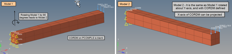
Figure 19. (a) Model 1: reference model (blank CORDM on PCOMPLS); (b) Model 2: Model 1 rotated by 90° about basic Y-axis (X-axis of CORDM on PCOMPLS can be projected
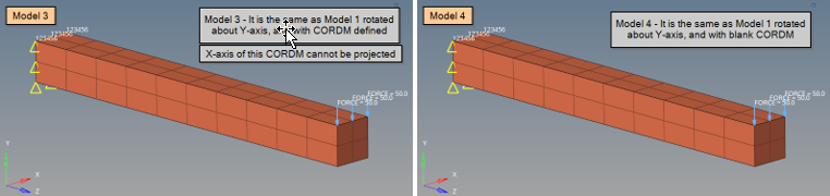
Figure 20. (a) Model 3: Model 1 rotated by 90° about basic Y-axis (different CORDM on PCOMPLS for which the X-axis cannot be projected); (b) Model 4: Model 1 rotated by 90° about basic Y-axis (blank CORDM on PCOMPLS)
- Model
1
model_1_blank_cordm.fem
PCOMPLS with blank CORDM
- Model 2
model_2_rotated_user_cordm.fem
Model 1 is rotated by 90° about Y-axis.
Additionally, PCOMPLS with CORDM defined referring to CORD2R (X-axis can be projected).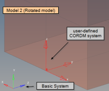
Figure 21. Projected X-axis of CORDM on PCOMPLS - Model 3
model_3_rotated_user_cordm.fem
Model 1 is rotated by 90° about Y-axis.
Additionally, PCOMPLS with CORDM defined referring to CORD2R (X-axis cannot be projected).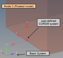
Figure 22. Non-Projected X-axis of CORDM on PCOMPLS - Model 4
model_4_rotated_blank_cordm.fem
Model 1 is rotated by 90° about Y-axis.
Additionally, PCOMPLS with blank CORDM.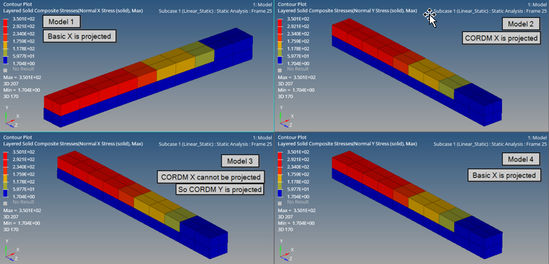
Figure 23. (a) Model 1: Blank CORDM on PCOMPLS (basic system); (b) Model 2: Rotated model with CORDM on PCOMPLS (local system with CORD2R); . (c) Model 3: Rotated model with CORDM on PCOMPLS (local system with CORD2R); (d) Model 4: Rotated model with blank CORDM on PCOMPLS (basic system)
As mentioned in Output, the elemental stress results are output in the Material Coordinate system for Continuum Shells. This can be illustrated by the four models listed above and in the interpretation of results (Figure 23).
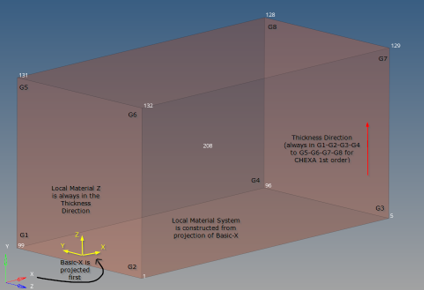
Figure 24. Element 208 (Model 1) Example. for blank CORDM, the X-axis of the Basic System is projected on the G1-G2-G3-G4 plane
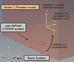
Figure 25. Model 2 projection of the CORDM X-axis and creation of local material system
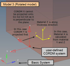
Figure 26. Model 3: projection of the CORDM X-axis is not possible - CORDM Y-axis is projected first. the local material system is now created from the projected Y and thickness direction Z
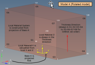
Figure 27. Model 4: CORDM is blank - the basic-X axis is projected onto the element. the local material system is then created based on this projected basic-X and the thickness direction which is the local material Z
| Generation of Local Material Coordinate Systems | |||
|---|---|---|---|
| Input Data | PSOLID | PCOMPLS | |
| CORDM field on Property PCOMPLS | CORDM=0 or blank (Basic System) | Basic System is used directly (No projection) |
The X-axis of the Basic System is projected. 3
The Z-axis is always in the Thickness Direction. 4 The Y-axis is the cross-product of these material Z and X-axes. 5 |
| CORDM=-1
(Elemental System) |
Elemental System1 is used directly (No projection) |
The X-axis of the Elemental System 6 is projected. 3
The Z-axis is always in the Thickness Direction. 4 The Y-axis is the cross-product of these material Z and X-axes. 5 |
|
| CORDM=Integer (User-defined System) |
User-defined System is used directly (No projection) |
The X-axis of the User-defined System is projected. 3
The Z-axis is always in the Thickness Direction. 4 The Y-axis is the cross-product of these material Z and X-axes. 5 |
|
| CORDM continuation line on element card (CHEXA) | CID=0
(Basic System) |
Basic System is used directly (No projection) |
The X-axis of the Basic System is projected. 3
The Z-axis is always in the Thickness Direction. 4 The Y-axis is the cross-product of these material Z and X-axes. 5 |
| CID=-1
(Elemental System) |
Elemental System 1 is used directly (No projection) |
The X-axis of the Elemental System6 is Projected. 3 The Z-axis is always in the Thickness Direction. 4 The Y-axis is the cross-product of these material Z and X-axes. 5 |
|
| CID
(User-defined System) |
User-defined System is used directly (No projection) |
The X-axis of the User-defined System is projected. 3
The Z-axis is always in the Thickness Direction. 4 The Y-axis is the cross-product of these material Z and X-axes. 5 |
|
| THETA/PHI | The Elemental System 1 is rotated based on
THETA/PHI
2 (No projection) |
The X-axis of the Rotated Elemental System 7 is projected. 3 The Z-axis is always in the Thickness Direction. 4 The Y-axis is the cross-product of these material Z and X-axes. 5 |
|
Interpretation of Results for Composites
Several composite-specific results are calculated for composite shell and continuum shell elements. Due to the specialized nature of these results, some explanation is provided regarding their meaning.
- Ply Stresses and Strains (CSTRESS and CSTRAIN
entries)
Classical lamination theory assumes two-dimensional stress-state in individual plies (so-called membrane state) for composite shells. The values of stresses and strains are calculated at the mid-plane of each ply, i.e. halfway between its upper and lower surface. For sufficiently thin plies, these values can be interpreted as representing uniform stress in the ply.
For composite shells, ply stresses and strains are calculated in coordinate systems aligned with ply material angles as specified on the corresponding composite property card. In particular, correspond to the primary ply direction, is orthogonal to it, and represents in-plane shear stress.
Composite materials typically have a low matrix Young’s modulus in comparison to the fiber modulus. Since the matrix is the bonding material in between plies, a shearing effect on the laminate is built up by the contributions of each interlaminar zone of the matrix. Because the longitudinal and transverse shear moduli is relatively lower than the longitudinal and transverse Young’s modulus, the effect of transverse shear stresses are important in composite panels than for isotropic plates. The theory behind the calculation of transverse shear stress is given in the subsequent section.
Ply stresses and strains can also be calculated at planes between the top and bottom planes of each ply. The NDIV field on the CSTRESS and CSTRAIN entries can be used to request the corresponding results for the required planes.
- Inter-laminar Stress
Inter-laminar bonding matrix usually has different material properties and stress-state than the individual plies. For composite shells, the primary stress that is of importance here is inter-laminar shear with two components: and . For continuum shells, in addition to interlaminar shear, interlaminar normal stress () at the interface between plies is also available.
- Failure Indices To facilitate prediction of potential failure of the laminate, failure indices are calculated for plies and bonding material. While there are several theories available for such calculations, their common feature is that failure indices are scaled relative to allowable stresses or strains, so that:
- the value of a failure index lower than 1.0 indicates that the stress/strain is within the allowable limits (as specified on the material data card), and
- a failure index above 1.0 indicates that the allowable stress/strain has been exceeded.
- according to the formula, some failure criteria (for example, Tsai-Wu and Hoffman) would produce the negative ply failure, depending on the problem.
Failure Criteria for Composite Laminated Shells
Hill's Theory of Ply Failure
The CRITERIA field on MATF or FT field of PCOMP/PCOMPP/PCOMPG should be set to HILL.
- The allowable stress in the ply material direction (1).
- The allowable stress in the ply material direction (2).
- The allowable in-plane shear stress.
On MAT8 entry, and , . If this suggestion is not adopted, warning messages will be output and the following rules will be applied: If , ; otherwise, , and similarly for and . For the interaction term, if , ; otherwise, .
On MATF entry, , ,
Hoffman's Theory of Ply Failure
The CRITERIA field on MATF or FT field of PCOMP/PCOMPP/PCOMPG should be set to HOFF.
On MAT8 entry, , , , ,
On MATF entry, , , , ,
Tsai-Wu Theory of Ply Failure
The CRITERIA field on MATF or FT field of PCOMP/PCOMPP/PCOMPG should be set to TSAI.
Where, is a factor to be determined experimentally.
On MAT8 entry, , , , , ,
On MATF entry, , , , ,
Maximum Strain Theory of Ply Failure
The CRITERIA field on MATF or FT field of PCOMP/PCOMPP/PCOMPG should be set to STRN.
- The allowable strain in the ply material direction (1).
- The allowable strain in the ply material direction (2).
- The allowable in-plane engineering shear strain.
On MAT8 entry, , , . The STRN field can be used to identify whether input values are stress or strain allowables.
On MATF entry, , , .
Maximum Stress Theory of Ply Failure
The CRITERIA field on MATF should be set to STRS.
- The allowable stress in the ply material direction (1).
- The allowable stress in the ply material direction (2).
- The allowable in-plane engineering shear stress.
On MATF entry, , , .
Bonding Material Failure
Where, is the allowable shear in the bonding material.
On PCOMP/PCOMPP/PCOMPG entry,
Hashin Failure Criteria
The CRITERIA field on MATF or FT field of PCOMP/PCOMPP/PCOMPG should be set to HASH.
The Hashin Failure criteria is calculated for four basic failure modes: in fiber tension, fiber compression, matrix tension, and matrix compression and the failure indices are output for all modes separately.
- Fiber Tension ()
(16) - Fiber Compression ()
(17) - Matrix Tension ()
(18) - Matrix Compression ()
(19)
- The allowable homogenized longitudinal tension strength of the composite.
- The allowable homogenized longitudinal compression strength of the composite.
- The allowable homogenized transverse tension strength of the composite.
- The allowable homogenized transverse compression strength of the fibers.
- The allowable homogenized longitudinal shear strength of the composite.
- The allowable homogenized transverse shear strength of the composite,
defined by the Hashin approximation:
(20) - The stress in the 1-direction.
- The stress in the 2-direction.
- The shear stress in 1-2 plane.
On MAT8 entry, , , , , .
On MATF entry, , , , , .
Puck Failure Criteria
The CRITERIA field on MATF or FT field of PCOMP/PCOMPP/PCOMPG should be set to PUCK.
The Puck failure criteria is calculated for two basic failure modes based on 2D plane stress, in fiber failure mode and inter-fiber failure mode. The failures indices are output separately for all these failure modes.
The allowable material data should be specified on the MATF Bulk Data Entry for Puck Failure Criterion. The corresponding failure indices are calculated as:
- Fiber Tension ()
(21) - Fiber Compression ()
(22)
- Mode A ()
(23) - Mode B ()
(24) - Mode C ()
(25)
- The allowable longitudinal tension strength.
- The allowable longitudinal compression strength.
- The allowable transverse tension strength.
- The allowable transverse compression strength.
- The allowable shear strength.
- The stress in the 1-direction.
- The stress in the 2-direction.
- The shear stress in 1-2 plane.
- The failure envelope factor 12(+).
- The failure envelope factor 12(-).
- The failure envelope factor 22(-).
On MATF entry, , , , , , , , .
The output results of failure mode for Hashin and Puck failure criterion are mutually exclusive. For example, a specified ply cannot fail due to tension and compression simultaneously. In such cases, the result plot for the other failure modes of the ply are not valid and this situation is represented by the notation – N/A, on the result plot.
Final Failure Index for Composite Element
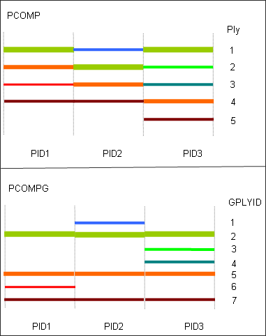
Figure 28. Comparison of Laminate Modeled with PCOMP and PCOMPG
Failure Criteria for Composite Anisotropic Solid and Continuum Shell Elements
- HILL3D
- PUCK3D
- HOFF3D
- TSAI3D
- HASH3D
- STRN3D
- STRS3D
- CNTZ3D
- HILL3D
- HOFF3D
- TSAI3D
- STRN3D
- STRS3D
The details of each failure criteria are presented in this section.
The normal stresses, , and shear stresses, , are in the material coordinate system (solid elements with MAT9/MAT9OR) or in fiber coordinate system (PCOMPLS).
Hill Criteria
On MATF, set CRITERIA to HILL3D.
or , depending on in tension or compression.
or , depending on in tension or compression.
or , depending on in tension or compression.
, , .
- V1
- V2
- V3
- V4
- V5
- V6
- V7
- V8
- V9
Hoffman Criteria
On MATF, set CRITERIA to HOFF3D.
- V1
- V2
- V3
- V4
- V5
- V6
- V7
- V8
- V9
Tsai-Wu Criteria
On MATF, set CRITERIA to TSAI3D.
- , ,
- Defined in MATF card as V10, V11 and V12, respectively.
Where, and the terms are the tensile stress limits in equal-biaxial tension tests.
- W1
- W2
- W3
W1 is the tension stress limit in equal-biaxial tests where the two tension loads are in directions 1 and 2. W1 is mandatory, while W2 and W3 are optional. If W2 and W3 are not specified, then they are set equal to W1. The definition of W2 and W3 is similar to W1. W2 is the tension stress limit in equal-biaxial tension tests where the two tension loads are in directions 2 and 3. W3 is the tension stress limit in equal-biaxial tension tests where the two tension loads are in directions 1 and 3.
- V1
- V2
- V3
- V4
- V5
- V6
- V7
- V8
- V9
- W1
- W2
- W3
If V10, V11, V12, W1, W2 and W3 are all blank, the coupling coefficients , , and are 0.0.
Maximum Strain Criteria
On MATF, set CRITERIA to STRN3D.
- Strain limit in direction. It can be taken as tension or compression strain limit, depending on the sign of corresponding normal strain ( = or ; = or ; and = or ).
- V1
- V2
- V3
- V4
- V5
- V6
- V7
- V8
- V9
In continuum shell elements (PCOMPLS), the above four criteria are available, , and . Also, the Hashin, Puck and Cuntze criteria can be used.
Maximum Stress Criteria
The CRITERIA field on MATF should be set to STRS3D.
,
- Stress limit in direction. It can be taken as tensile or compressive stress limit, depending on the sign of corresponding normal stress (= or , = or , and = or ).
On the MATF Bulk Data Entry, V1 = , V2 = , V3 = , V4 = , V5 = , V6 = , V7 = , V8 = , and V9 = .
In continuum shell elements (PCOMPLS), the above five criteria are available. Besides, three additional criteria, which are only available for PCOMPLS can be used: Hashin, Puck and Cuntze.
Hashin Criteria
On MATF, set CRITERIA to HASH3D.
- Fiber Tension
- Fiber Compression
- Matrix Tension
- Matrix Compression
- Fiber Tension ()
(33) Where, α is a user-defined empirical parameter. This is used to define the contribution of transverse shear stress taken into account in the Fiber Tension mode. The coefficient α is automatically set as 1.0, if W1 is left as blank in the MATF card.
- Fiber Compression ()
(34) - Matrix Tension ()
(35) - Matrix Compression ()
(36)
- V1
- V2
- V3
- V4
- V5
- V6
- V7
- V8
- V9
- W1
- which is used in fiber tension failure check
Puck Criteria
On MATF, set CRITERIA to PUCK3D.
- Fiber Tension Mode ()
(37) - Fiber Compression Mode ()
(38) - Inter-Fiber check 1 ()
(39) - Inter-Fiber check 2 ()
(40) Where,
- , , , and
- Coefficients for the envelope of failure curve, and they should be provided by users in the MATF card as W1, W2, W3, and W4, respectively.
A search on the critical failure plane is performed automatically from -90° to 90° at every 1°.
- V1
- V2
- V3
- V4
- V5
- V6
- V7
- V8
- V9
- W1
- W2
- W3
- W4
Cuntze Criteria
On MATF, set CRITERIA to CNTZ3D.
- FF1
(41) - FF2
(42) - IFF1
(43) - IFF2
(44) - IFF3
(45)
Where, .
Where, is the interaction exponent.
- V1
- V2
- V3
- V4
- V5
- V6
- V7
- V8
- V9
- W1
- (Default = 0.15)
- W2
- (Default = 1.0)
- W3
- (Default = 2.6)
Interlaminar Shear Failure Index
Where, is user-defined in the SB field on the PCOMPLS card.