2D curve: about
Introduction
The various quantities calculated in Flux can be graphically represented as curves.
One can distinguish two types of curves:
- The curves called « local » with regard to the representation of a local quantity in function of position
- The curves called « temporal » or « parametric » with regard to the representation of a quantity in function of a parameter or of time.
2D Curves (Path) and (I/O Parameter)
The two types of curves called in the software 2D Curve (Path) and 2D Curve (I/O Parameter) are presented in the table below.
| Type | Description | |
|---|---|---|
| 2D Curve (path) | curve along a path | Graphic representation of one (or more) local quantity(s) in function of the position along a path (previously created) |
| 2D Curve (I/O Parameter) | curve in function of an I/O parameter | Graphic representation of one (or more) local or global quantity(s) in function of a variable quantity (I/O parameter) |
Operation
The general process comprises the following phases:
| Phase | Description |
|---|---|
| 1 |
The user creates a 2D curve defining:
|
| 2 |
The software creates the 2D curve i.e.:
|
| 3 |
The user can:
|
Vocabulary
Attention, it is necessary to define the vocabulary associated with the objects manipulated in Flux.
In this document, we name:
- curve or elementary curve, a curve (in the usual sense of the term), i.e. the representation of the evolution law of a phenomenon
- 2D Curve*, the entity Flux that regroups one or more elementary curves
Note: * This can be the 2D Curve (path) or the 2D Curve (I/O Parameter) , which are two
types of distinct entities in the data tree.
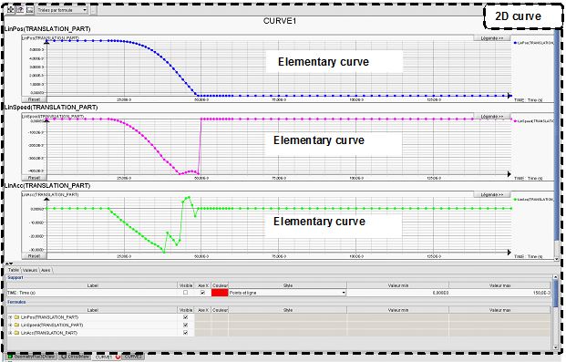
Example
The notions of 2D curve and of elementary curves are explained in the example below.
The 2D curve called CURVE1 regroups the following elementary curves:
- LinPos(TRANSLATION_PART)
- LinSpeed(TRANSLATION_PART)
- LinAcc(TRANSLATION_PART)