ACU-T: 3101 Transient Conjugate Heat Transfer in a Mixing Elbow
Prerequisites
This tutorial provides you instructions for running a transient simulation of a 3D turbulent flow with conjugate heat transfer in a mixing elbow using HyperWorks CFD and AcuSolve. You should have already run through the ACU-T: 3100 Conjugate Heat Transfer in a Mixing Elbow tutorial and have a basic understanding of HyperWorks CFD and AcuSolve. The HyperWorks introductory tutorial, ACU-T: 1000 Basic Flow Set Up, gives a basic introduction to HyperWorks, AcuSolve, and HyperView.
Prior to running through this tutorial, click here to download the tutorial models. Extract ACU-T3101_MixingElbowTransient.hm from HyperWorksCFD_tutorial_inputs.zip.
Problem Description
This problem is divided into two components, a steady state solution and a transient solution. The schematic of the steady state component is shown below.

Figure 1.
The diameter of the large inlet is 0.1 m, the inlet velocity (v) is 0.4 m/s and the temperature (T) of the fluid entering the large inlet is 295 K. The diameter of the small inlet is .025 m, the velocity is 1.2 m/s, and the temperature of the fluid entering the small inlet is 320 K. The pipe wall has a thickness of 0.005 m. The fluid in this problem is water and the pipe walls are made of stainless steel with a density of 8030 kg/m3, a conductivity of 16.2 W/m-K, and a specific heat of 500 J/kg-K.
The model file for the steady state part of the problem is provided as the input file. Once the steady state solution is computed, it is projected on to the mesh and used as the initial state for the transient simulation. The starting point for the transient portion of the problem is shown schematically in the figure below.
Figure 2.
At 0.2s into the simulation, a cold slug of water is injected at both the inlets and the temperature is ramped down to 283.15 K starting from 0.2 s to 0.4 s. Then it is maintained constant at 283.15 K for 1 sec and then ramped up to initial states from 1.4s to 1.6s. Given a flow path of 0.6356 m, the transit time for the slug is approximately 1.6s. Therefore, our simulation time should be at least 3.2 s to factor in the duration of the slug and transit time. The total simulation time will be 4.5s to allow time for the thermal conditions to return to a steady state.
The temperature change at the large inlet is from 295 K to 283.15 K. At the small inlet, the temperature changes from 320 K to 283.15 K. The ratio of the cold slug temperature to the initial temperature of the large inlet flow is 0.9598. The ratio of the cold slug temperature to the initial temperature of the small inlet flow is 0.8848. These values will be used in creating multiplier functions to model the transient temperatures at the inlets.
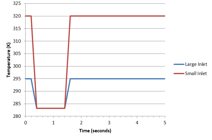
Figure 3.
Start HyperWorks CFD and Open the HyperMesh Database
-
From the Home tools, Files tool group, click the Open Model tool.

Figure 4.The Open File dialog opens.
Run the Steady State Simulation
In this step, you will run the steady state simulation with the input file provided.
-
From the Solution ribbon, click the Run tool.

Figure 5.The Launch AcuSolve dialog opens. -
Click Run to launch AcuSolve.
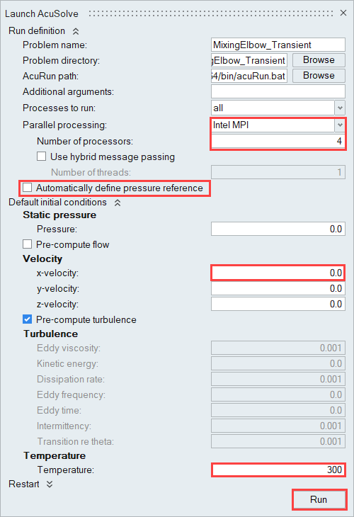
Figure 6. -
Once the solver run is complete, close the Run Status
dialog.
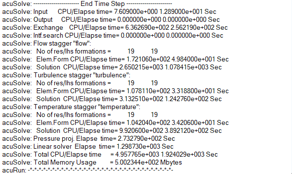
Figure 7.
Set the Transient Simulation Parameters
-
From the Flow ribbon, click the Physics tool.

Figure 8.The Setup dialog opens. -
Under the Physics models setting:
- Set Time marching to Transient.
- Set the Time step size to 0.053 and the Final time to 4.5.
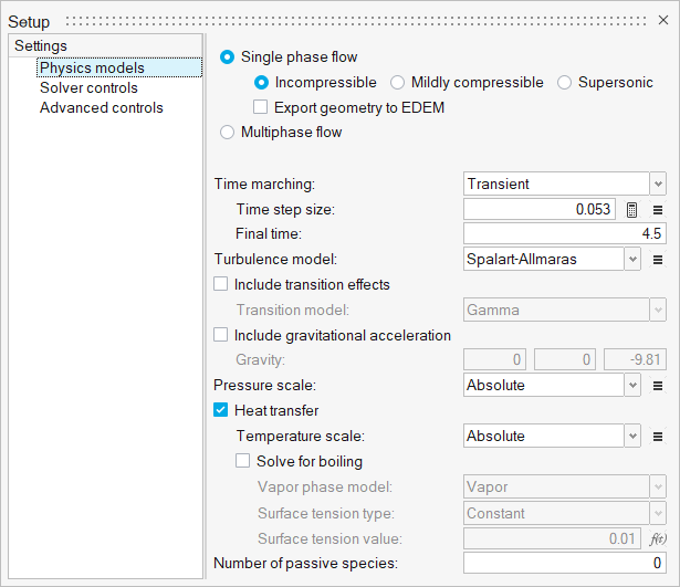
Figure 9. -
De-activate the Flow and
Turbulence equations.
By turning these options off, AcuSolve will not update the solution to these equations. Instead, the current flow and turbulence values (generated from the steady state solution for this tutorial) will be used throughout the simulation, and AcuSolve will only solve for the temperature field.
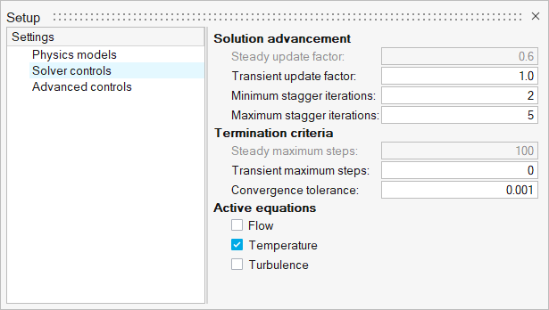
Figure 10.
Specify the Transient Inflow Boundary Conditions
-
From the Flow ribbon, Profiled
tool group, click the Profiled Inlet tool.

Figure 11. -
In the modeling window Boundaries legend, right-click
on Large Inlet and select Edit
from the context menu.
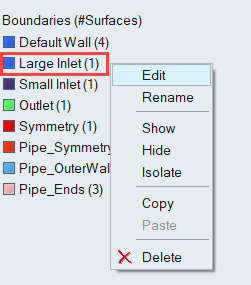
Figure 12. -
In the microdialog, click multiplier function drop-down
menu next to Temperature and select Create new.
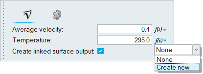
Figure 13. -
In the dialog that appears, edit the name of the multiplier function by
clicking
 in the
top-left corner. Set the name to Large Inlet.
in the
top-left corner. Set the name to Large Inlet.
-
Click
 four times
to add four new rows to the bottom of the table.
four times
to add four new rows to the bottom of the table.
-
Enter the table values for the multiplier function as shown in the image
below.
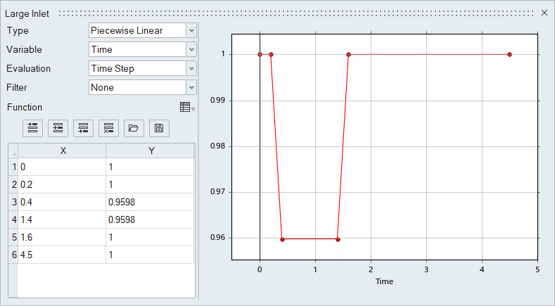
Figure 14. -
On the guide bar, click
 to execute the command and remain in the
tool.
to execute the command and remain in the
tool.
-
In the dialog that appears, edit the name of the multiplier function by
clicking in the
top-left corner. Set the name to Small Inlet.
-
Click four times
to add four new rows to the bottom of the table.
-
Enter the table values for the multiplier function as shown in the image
below.
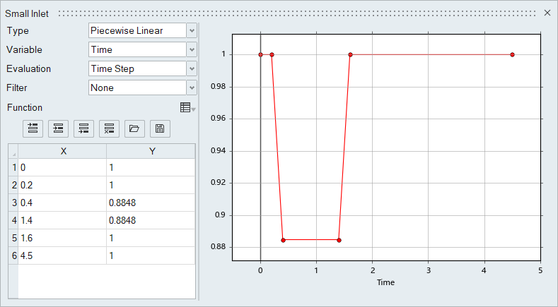
Figure 15. -
On the guide bar, click
 to execute
the command and exit the tool.
to execute
the command and exit the tool.
Compute the Solution
Define Nodal Outputs
-
From the Solution ribbon, click the Field tool.

Figure 16.The Field Output dialog opens. -
Activate the Write initial conditions option and set the
Time step interval to 3 for the Solution variables.
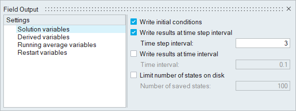
Figure 17.
Launch AcuSolve
-
From the Solution ribbon, click the Run tool.
Figure 18.The Launch AcuSolve dialog opens. -
Click Run to start the transient run.
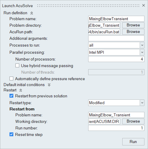
Figure 19.
Post-Process the Results with HW-CFD Post
-
Isolate the Pipe_Symmetry and
Symmetry flow boundaries in the Post Browser.
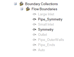
Figure 20. -
Click the Boundary Groups tool.

Figure 21. -
Activate the Legend toggle and click
 to reset the range.
-
Click
 and set the Colormap Name to Rainbow
Uniform.
and set the Colormap Name to Rainbow
Uniform.
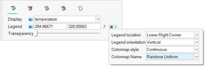
Figure 22. -
Click
 on the guide bar.
-
Click
 at the bottom of the modeling window to view an animation of the transient flow
with respect to the temperature contour.
at the bottom of the modeling window to view an animation of the transient flow
with respect to the temperature contour.
Figure 23. -
Save the animation.
- Go to .
-
Click
 on the toolbar.
- Uncheck Include mouse cursor.
- Set the frame rate to 50.
-
Click
 on the toolbar then drag over the area you
want to record.
on the toolbar then drag over the area you
want to record.
-
Click
 to start recording and the same button to
stop recording.
to start recording and the same button to
stop recording.
- Name the file and save it.
Summary
In this tutorial, you learned how to set up and run a transient conjugate heat transfer simulation using HyperWorks CFD and AcuSolve. You started by importing the input file, which had the conjugate heat transfer setup for the steady state run. Once the steady state solution was computed, you set the transient simulation parameters and applied the transient conditions at the inlets. Once the transient solution was computed, you post-processed the results using the Post ribbon.