ACU-T: 3110 Exhaust Manifold Conjugate Heat Transfer - CFD Data Mapping
Prerequisites
Prior to starting this tutorial, you should have already run through the introductory tutorial, ACU-T: 1000 Basic Flow Set Up, and have a basic understanding of HyperWorks CFD and HyperView. To run this simulation, you will need access to a licensed version of HyperWorks CFD and AcuSolve.
Prior to running through this tutorial, click here to download the tutorial models. Extract ACU-T3110_acuOptiStruct.hm from HyperWorksCFD_tutorial_inputs.zip.
Since the HyperWorks CFD database (.hm file) contains meshed geometry, this tutorial does not include steps related to geometry import and mesh generation.
Problem Description

Figure 1. Schematic of Exhaust Manifold
The diameter of the inlets is 0.036 m; the inlet velocity (v) is 8.0 m/s; and the temperature (T) of the fluid entering the inlets is 700 K. The diameter of the outlet is 0.036 m. The pipe wall has a thickness of 0.003 m and the flanges have a thickness of 0.01 m.
The combustion mixture enters the inlets and heat is transferred through conduction inside the manifold. The heat transfer causes deformations and stress in the manifold body which can be simulated using OptiStruct.
- Density (ρ)
- 1.225 kg/m3
- Viscosity (μ)
- 1.781 * 10-5 kg/m-s
- Specific Heat (Cp)
- 1005 J/kg-K
- Conductivity (k)
- 0.0251 W/m-K
- Density (ρ)
- 8000 kg/m3
- Specific Heat (Cp)
- 500 J/kg-K
- Conductivity (k)
- 16.2 W/m-K
For the HyperWorks CFD simulation, the variation in material properties of air with temperature is ignored.
The HyperWorks CFD simulation will be set up to model steady state heat transfer to determine the temperature and pressure distribution on the walls of the manifold.
The nodal surface output needs to be activated for all the surfaces in order to create the OptiStruct input deck from the acuOptiStruct command.
The temperature distribution and forces on the wetted surfaces are used by OptiStruct to calculate the deformations and stress in the solid body.
- -solids
- Input name for the solid body/bodies where conduction heat transfer would take place.
- -den
- Density values for the solid body/bodies.
- -spcsurfs
- List of surfaces where boundary condition constraints need to be specified.
- -spcsurfsdof
- List of degrees of freedom for the surfaces.
- -spcsurfsdofvals
- List of degrees of freedom values for the surfaces which is zero by default.
- -type
- Stress analysis type for the OptiStruct solver.
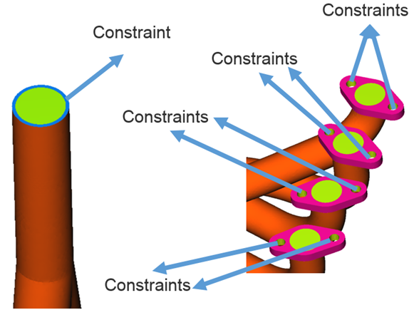
Figure 2.
The stress analysis type is selected as steady linear where the deformations are in the elastic range; that is, the stresses, σ, are assumed to be linear functions of the strains, ε, Hooke's law can be used to calculate the stresses.
Start HyperWorks CFD and Open the HyperMesh Database
-
From the Home tools, Files tool group, click the Open Model tool.

Figure 3.The Open File dialog opens.
Validate the Geometry
The Validate tool scans through the entire model, performs checks on the surfaces and solids, and flags any defects in the geometry, such as free edges, closed shells, intersections, duplicates, and slivers.
Figure 4.
Set Up Flow
Set Up the Simulation Parameters and Solver Settings
-
From the Flow ribbon, click the Physics tool.

Figure 5.The Setup dialog opens. -
Under the Physics models setting:
- Set Time marching to Steady.
- Select Spalart-Allmaras as the Turbulence model.
- Activate the Include gravitational acceleration and Heat transfer options.
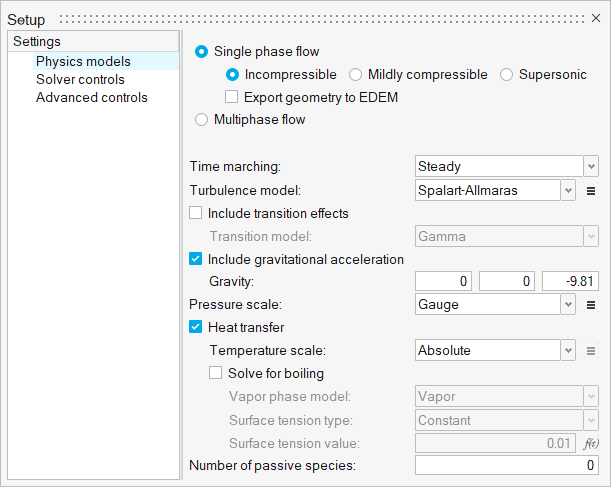
Figure 6. -
Verify the following parameters.
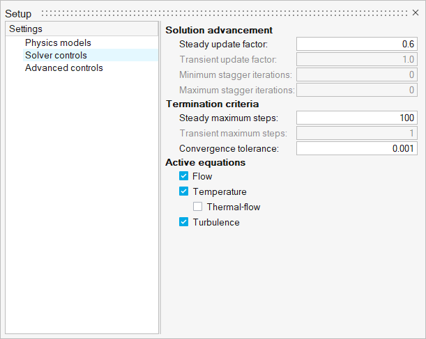
Figure 7.
Assign Material Properties
-
From the Flow ribbon, click the Material tool.

Figure 8. -
In the microdialog, select Stainless steel
(304) from the drop-down.
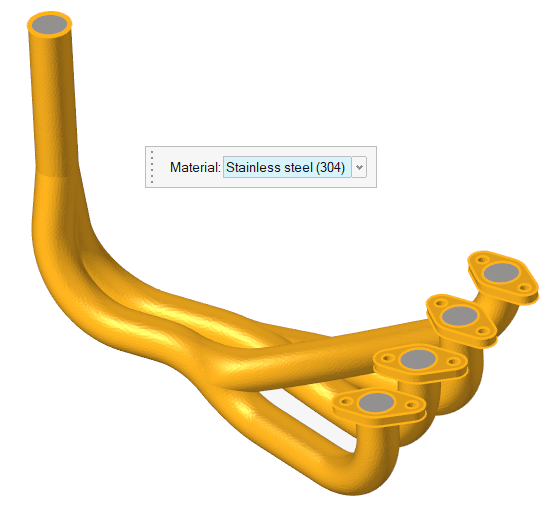
Figure 9. -
On the guide bar, click
 to execute the command and remain in the
tool.
to execute the command and remain in the
tool.
-
In the microdialog, select Air
from the drop-down.
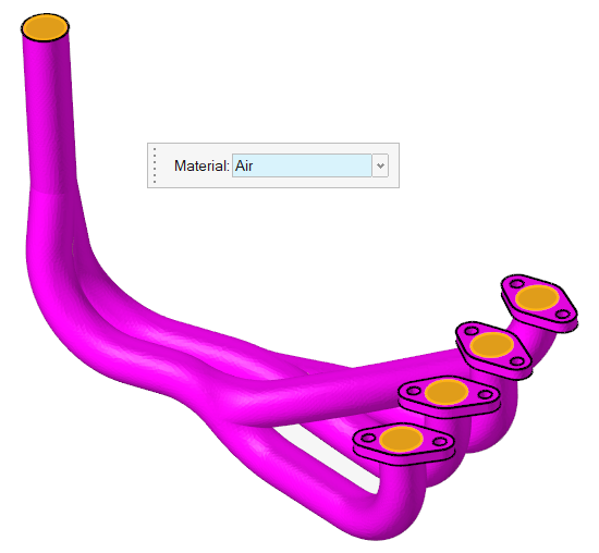
Figure 10. -
On the guide bar, click
 to execute
the command and exit the tool.
to execute
the command and exit the tool.
Assign the Flow Boundary Conditions
-
From the Flow ribbon, click the Constant tool.

Figure 11. -
Select the manifold inlets highlighted in the figure below.
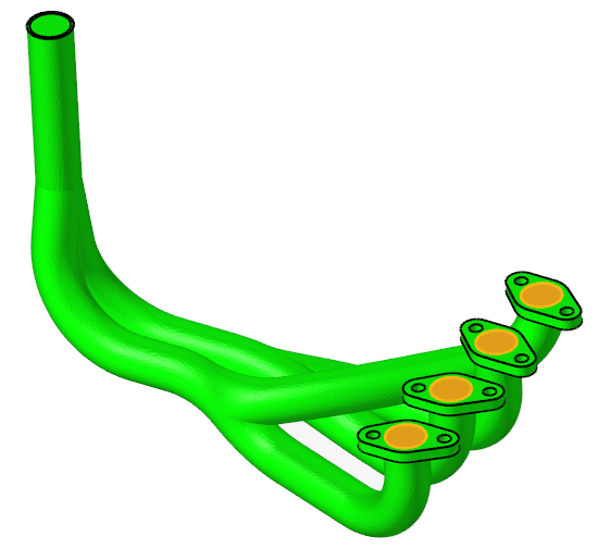
Figure 12. -
In the microdialog, set the Inflow velocity type to
Normal, the Normal velocity to
8.0 and the Temperature to
700.
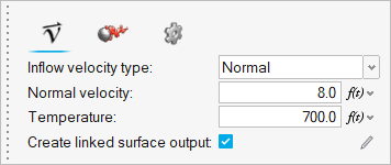
Figure 13. -
Click the Turbulence tab in the microdialog. Set the input type to Viscosity
Ratio and the viscosity ratio value to
40.
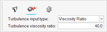
Figure 14. -
On the guide bar, click
to execute
the command and exit the tool.
-
Click the Outlet tool.

Figure 15. -
Select the face highlighted in the figure below and verify that both the static
pressure and the pressure loss factor are set to 0.
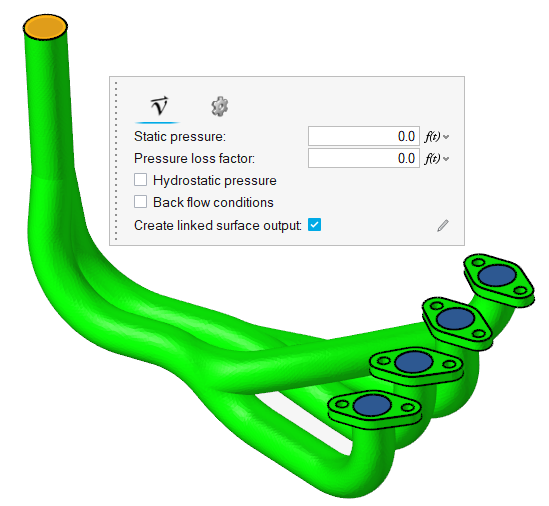
Figure 16. -
Click
 on the guide bar.
-
Click the No Slip tool.

Figure 17. -
Select the wall flanges.
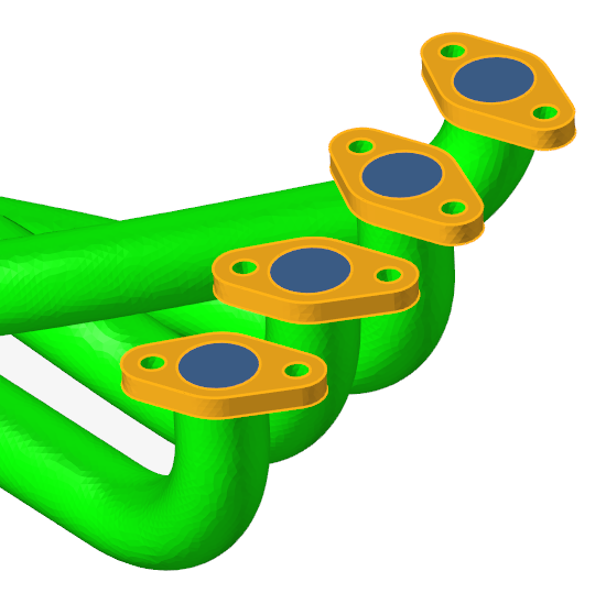
Figure 18.Note: Make sure you select the bottom and side surfaces of the flanges. In total, 12 surfaces should be selected. -
In the microdialog, click the
Temperature tab, set the Convective heat coefficient
to 100, and the Convective heat reference temperature to
303.
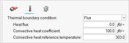
Figure 19. -
Click
 on the guide bar.
-
Select the flange bolts.
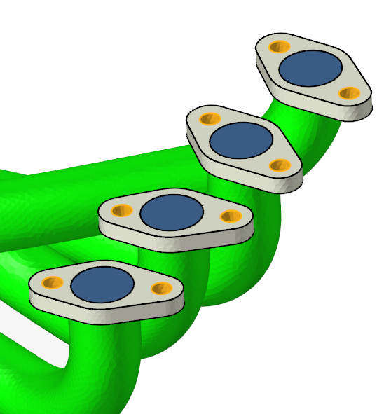
Figure 20. -
Click on the guide bar.
-
Select the outlet end.
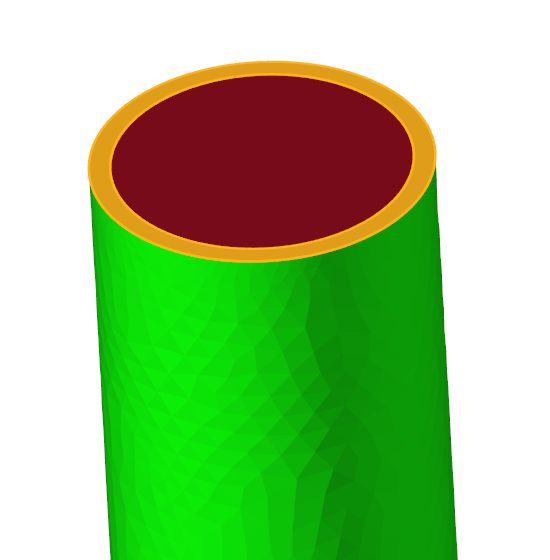
Figure 21. -
Click on the guide bar.
-
Select the outer solid walls.
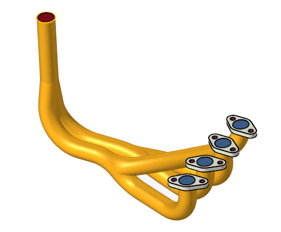
Figure 22. -
Click on the guide bar.
-
Hide all previously assigned surfaces then select the remaining surface.
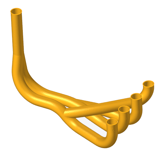
Figure 23. -
Check that default values are assigned to the thermal boundary
conditions.
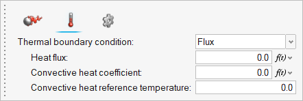
Figure 24. -
Click on the guide bar.
Link Surface Output
-
In the microdialog, activate the checkbox for
Create linked surface output.
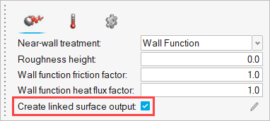
Figure 25. -
Click
 to edit the values.
-
Set the following linked surface output settings for the inlets, the outlet,
and all the wall surfaces (Outlet_End, Flange_Bolts, Outer_Solid_Walls,
Fluid_Walls).
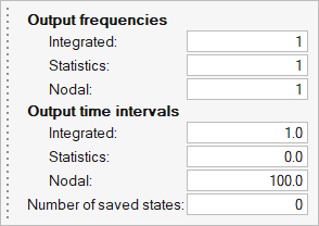
Figure 26.
Run AcuSolve
-
From the Solution ribbon, click the Run tool.

Figure 27. -
Leave the remaining options as default and click
Run to launch AcuSolve.
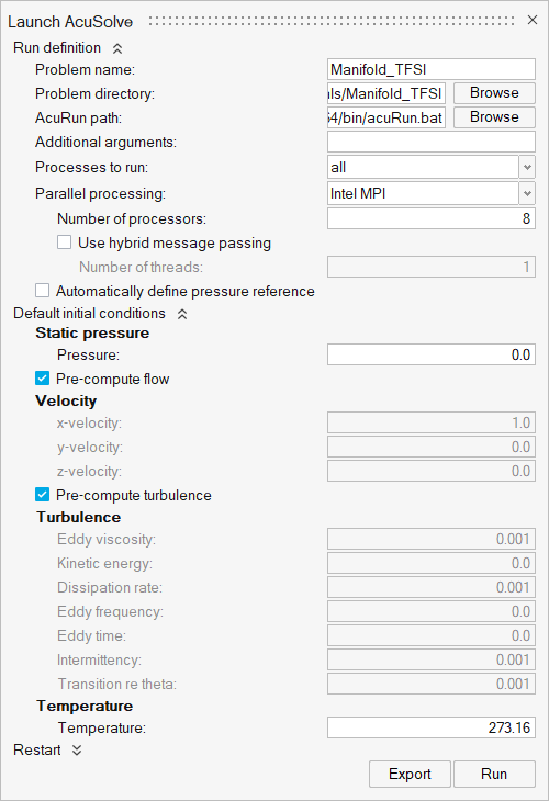
Figure 28.
Run acuOptiStruct
-
Execute the following command:
acuOptiStruct -solids “Exhaust Steel” -spcsurfs “Flange_Bolts – Output”,”Outlet_End – Output” -spcsurfsdof 123456,123456 -spcsurfsdofvals 0,0 -type sl
You should see a similar output as below when the command executes successfully.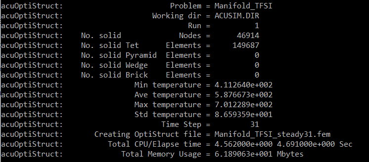
Figure 29.
Run OptiStruct
-
Click
 next to Input file(s).
-
Select the .fem file.
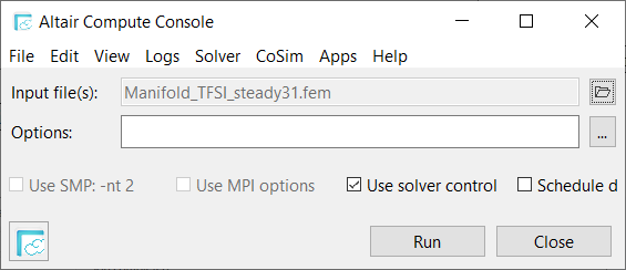
Figure 30. -
Click Run to run the case.
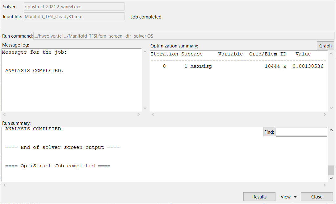
Figure 31.
Post-Process the Results with HW-CFD Post
-
Click the Boundary Groups tool.

Figure 32. -
Click
 and set the Colormap name to Rainbow
Uniform.
and set the Colormap name to Rainbow
Uniform.
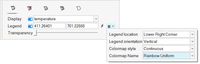
Figure 33. -
Click on the guide bar.
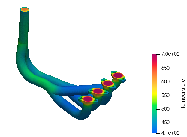
Figure 34. -
Click and set the Colormap name to Rainbow
Uniform.
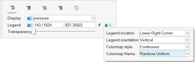
Figure 35. -
Hide all other flow boundaries.
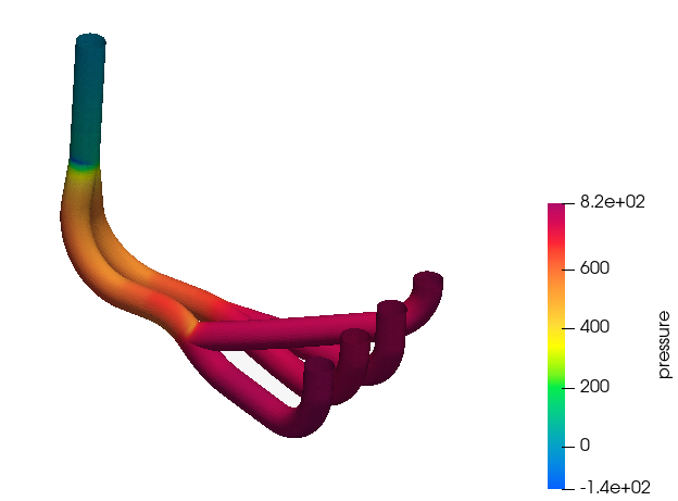
Figure 36.
Post-Process the OptiStruct Results with HyperView
-
In the Load model and results panel, click
 next
to Load model.
next
to Load model.
-
Click
 on the Results toolbar to open the Contour panel.
-
Click Apply to plot the displacement magnitude
contours.
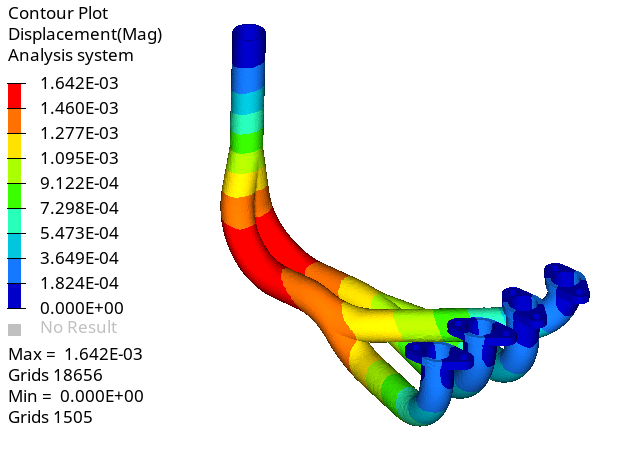
Figure 37. -
Click Apply.
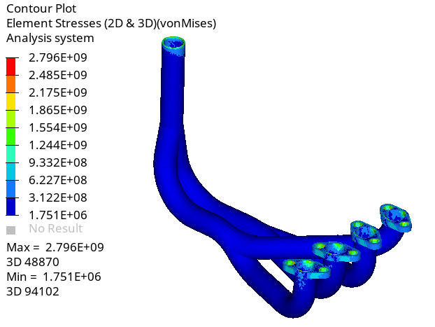
Figure 38.
Summary
In this tutorial, you learned how to set up a conjugate heat transfer problem using HyperWorks CFD and solve it using AcuSolve. Once you computed the solution, you used acuOptiStruct to generate the input deck for OptiStruct. Once the solution for the structural analysis was computed, you post-processed the results using HyperWorks CFD post and HyperView and created contour plots of Temperature, Pressure, Displacement, and Stress.