NVH analysis in OptiStruct with data setting in HyperMesh
Introduction
- How to make the physical data setting in HyperMesh
- How to run a frequency response analysis in OptiStruct
- How to make the post-processing in HyperView
Data setting in HyperMesh for OptiStruct analysis
- By manually modifying the files (mesh file, forces file) to import it directly into OptiStruct by using the include technology, without using HyperMesh
- By doing the data setting in HyperMesh
In this document, the following parts describe the second way which is more dedicated for beginner users.
The OptiStruct analysis which is done here is a frequency response analysis.
At the end, the post-processing in HyperView is presented.- Rename the component faces to
^faces and turn it to hidden mode (to ignore it in
the following steps). Make stator component visible.
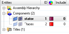
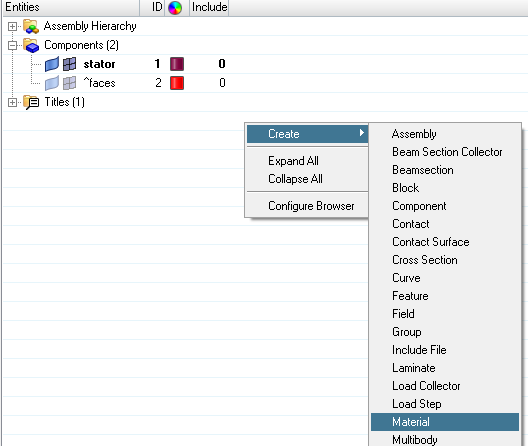
- Create the associated material to stator component. Here steel material is created:
- On the model area: right click on the blank space /
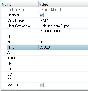
- The following 3 mechanical properties are defined for isotropic
material (E=Young modulus, Nu=Poisson Ratio, Rho=density):
- On the model area: right click on the blank space /
- Create a property to support 3D elements with a PSOLID
card image and define the material as steel. Assign it to the component:
- As for the material: right click in the model area / .
- Choose the following data:
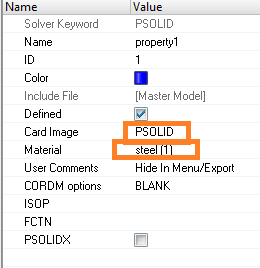
- Assign the property to the stator component: click on stator and choose property 1 in the window at the bottom
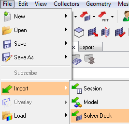
- Import forces file:
- Import solver deck:
 Verify the two following options to avoid the IDs re-numbering:
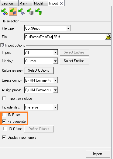
All loads created in Flux are imported in HyperMesh
- Import solver deck:
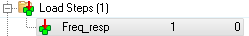
- Create the Load step which defines the OptiStruct analysis parameters:
- As for material and property, right click on Model area /
- Rename the load step to Freq_resp for
example
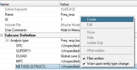
- Choose Analysis type: Freq. resp (modal)
- Choose DLOAD (the selection window opening can
take a while):
- Global dynamic load case or First component dynamic load case or Second component dynaminc load case
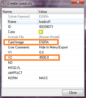
- Create a new METHOD(STRUCT) by right click /
Create on the corresponding field
- Choose the Card Image: EIGRA which allows performing eigenvalue analysis
- Choose V2 value which corresponds to the
maximum frequency to study. In general, the chosen value is 1.5
times the maximum frequency exported from Flux
- Choose FREQ (the selection window opening can
take a while):
- Choose List of frequencies
- It is advised to modify RESVEC parameter to
No in order to limit the used memory and the
solving time:
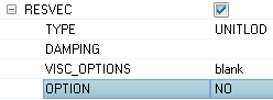 注: keeping the option to YES is more accurate but the computation time becomes non-industrial. Please refer to the residual vectors computation help section for more information
 - Choose the output to display after solving. For example: the DISPLACEMENT, the STRESS, the imported forces which corresponds to OLOAD keyword, etc.
- Damping Creation:
If you want to introduce global damping you can use the PARAM,G parameter:
The PARAM card can be access by the menu:
PARAM card appears in the model datatree: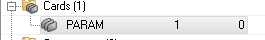
- Choose G which corresponds to the critical damping ration multiplied by 2. Here we choose G=0.04
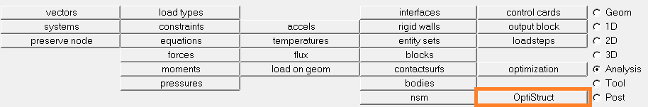
- Solve the OptiStruct problem:
- Open the Analysis panel below the graphic and
click on OptiStruct
 The following window is opened:
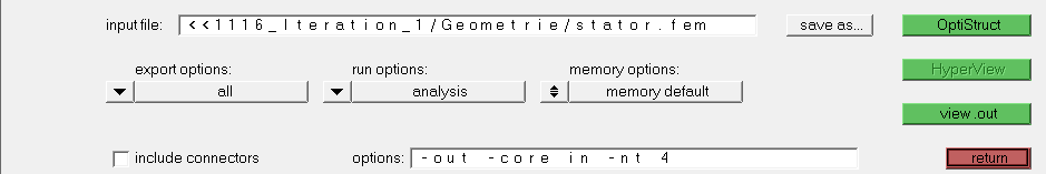
-
注: All the set-up model will be saved in the file .fem specified in the input file
- The export options must be set to all
- The run option must be set to analysis
- In the options, enter –out –core in
–nt 4 (the spaces must be respected).
Please refer to help section for solver options definition
- Click on OptiStruct to solve the problem
A window is opened after a short time. It displays the solving steps and the error messages if the problem can’t be solved. When the solving finishes, at the end the window displays Job completed. As a remark, to stop the solving, click on abort.
- Open the Analysis panel below the graphic and
click on OptiStruct
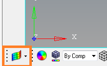
- Open HyperView to post-process.In HyperMesh Desktop, choose the following icon:
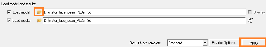
- Load the .h3d file which was automatically generated during the solving
and included all the data results and click on
Apply
- Load the .h3d file which was automatically generated during the solving
and included all the data results and click on
Apply
- To post-process in HyperView, use the following bar below the graphic:
 The subcase and the studied frequency can be chosen on the following fields on left side above the model tree:
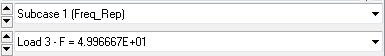
- The icon
 allows the user to review the contours requested:
 - Select Displacement/ Magnitude to review the displacements:
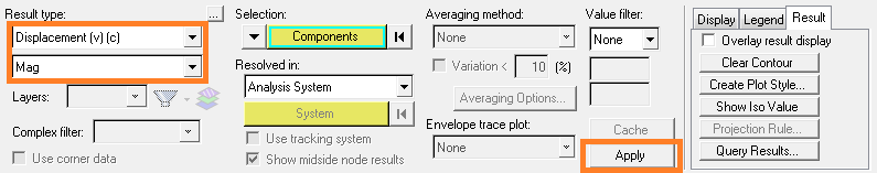
Select Stress VonMises to review the stresses computed using the invariant VonMises approach.
Please note that the stresses you are postprocessing are phase dependent.
To get the maximum VonMises stress over the phase you can use the derived results tool
with the operator scalarextract
tool
with the operator scalarextract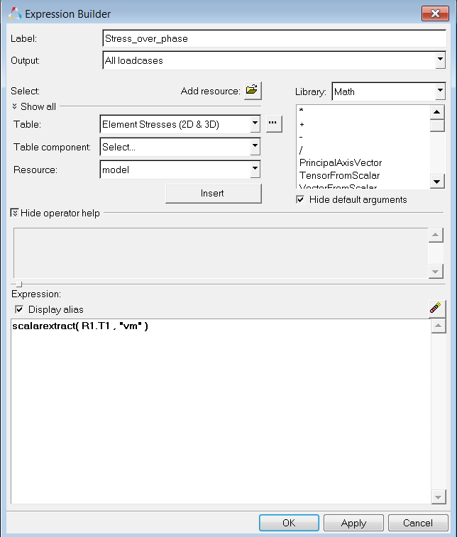
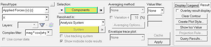
The R1.T1 corresponds to the Stresses tensor.
To review the contour of these VonMises stress over phase please make sure to turn the complex filter to mag: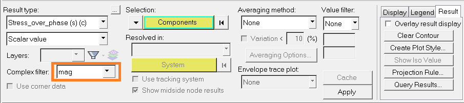
- Control of animation
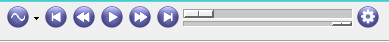
The second sliding bar allows you to slow down the animation.
The wheel icon on the right allows you to manage the animation steps thanks to the angular increment: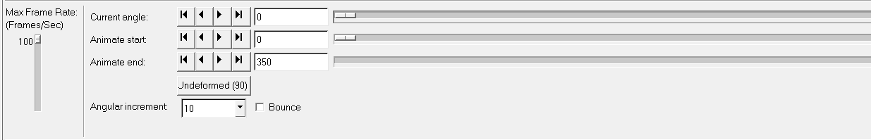
- You can also review the applied loads on 1 particular node: To do that, select the Applied Loads in the contour tool:
Set the angular increment to 5 degrees.
Launch the animation over at least 1 phase.
Open the Measures tool
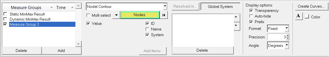
Add a measure with the Add button and select the nodal Contour in the pulldown menu.
Select the node of interest and click on Create Curves: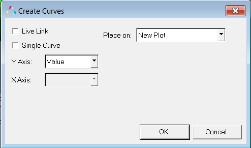
Click OK in this new popup window
A new window appears with the force vs phase graph: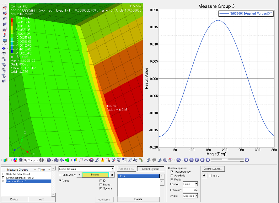
- The icon