Exercise 1: Define Model Data for the Seat Impact Analysis
In this exercise, you will define and review model data for a LS-DYNA analysis of a vehicle seat impacting a rigid block. The seat and block model is shown in Figure 1.
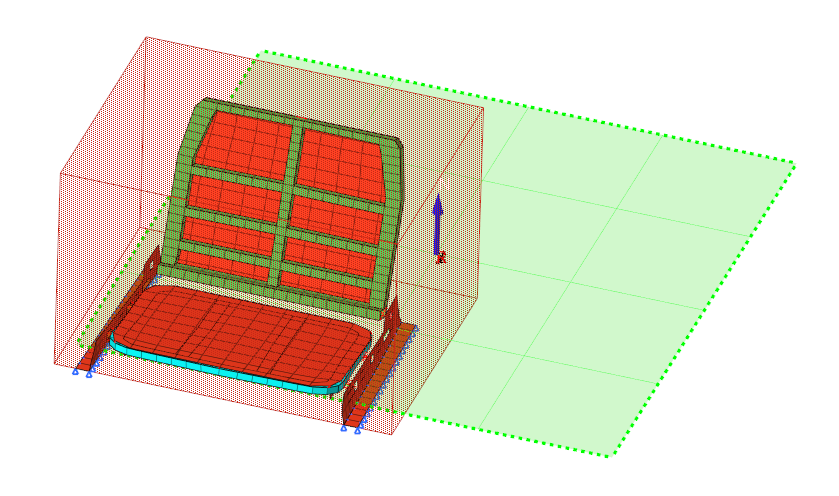
Figure 1.
Load the LS-DYNA User Profile
In this step, you will load the LS-DYNA user profile in Engineering Solutions.
- Start Engineering Solutions Desktop.
- In the User Profile dialog, set the user profile to LsDyna.
Retrieve the Engineering Solutions File
In this step, you will open the model file in Engineering Solutions.
-
Open the model file by completing one of the following options.
- Click from the menu bar.
- Click
 on the Standard toolbar.
Create an XY Plot
In this step, you will create an XY plot.
-
Set plot type to standard as seen in Figure 2.
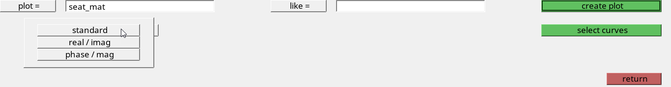
Figure 2.
Create Two Stress-Strain Curves
In this step, you will input data from a file to create two stress-strain curves.
-
Click input.
Engineering Solutions creates two curves, and names them 0.001 and 0.004 as seen in Figure 3.
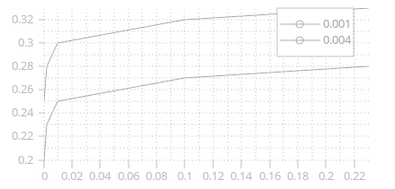
Figure 3.
Create a Dummy XY Curve
In this step, you will create a dummy XY curve to be used to create a *DEFINE_TABLE.
-
In the y = field, enter {0.4, 0.4}.
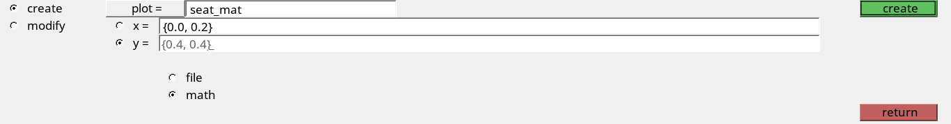
Figure 4. -
Click create.
Engineering Solutions creates a curve in the seat_mat plot, and names it curve3 as seen in Figure 5.
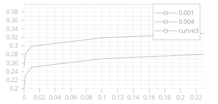
Figure 5.
Create a *DEFINE_TABLE
In this step, you will create a *DEFINE_TABLE from the dummy curve created in Create a Dummy XY Curve.
-
In the Model Browser, Curve folder, click
curve3.
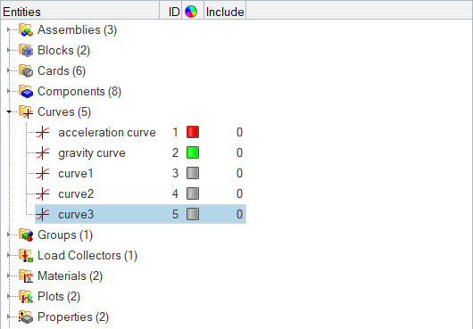
Figure 6.The Entity Editor opens, and displays the curve's corresponding data. -
In the Data: VALUE row, click
 .
.
-
In the ArrayCount dialog, enter
0.001 in the strain rate VALUE(1) field and
0.004 in the strain rate VALUE(2) field.
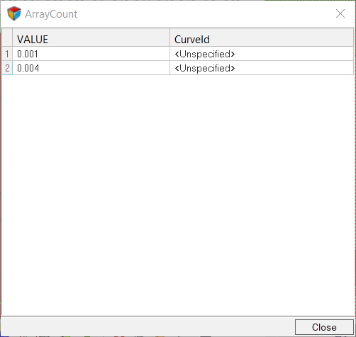
Figure 7. -
In the CurveId(1) field, click .
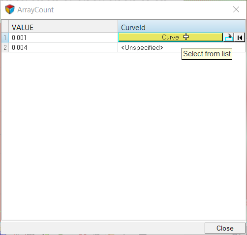
Figure 8. -
In the Select Curve dialog, select
curve1 and then click OK.
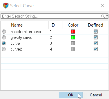
Figure 9. -
Click Close.
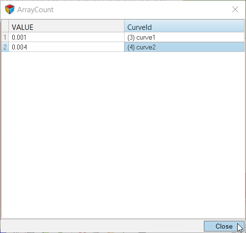
Figure 10.
Create a Non-Linear Material
In this step, you will create a non-linear material (*MAT_PIECEWISE_LINEAR_PLASTICITY).
-
In the Solver Browser, right-click and select from the context menu.
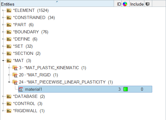
Figure 11.Engineering Solutions creates and opens a new material in the Entity Editor. -
Click LCSS and then click
curve.
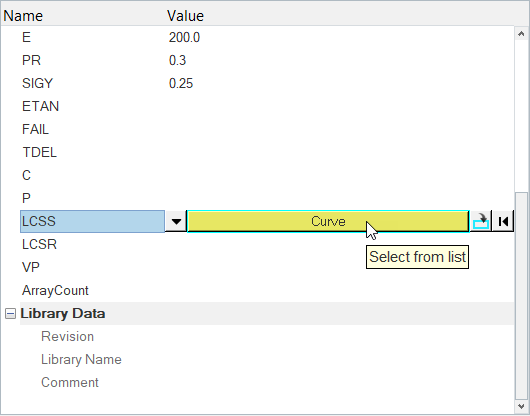
Figure 12. -
In the Select Curve dialog, select
curve3 and then click OK.
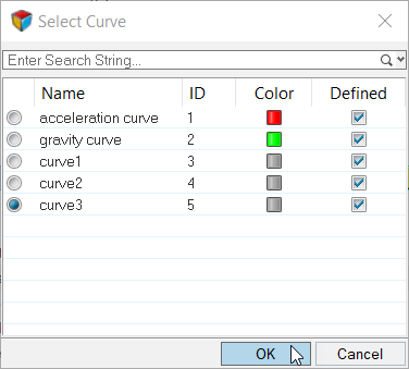
Figure 13.
Update the Components with the New Material
In this step, you will update the base_frame and back_frame components with the non-linear material created in Create a Non-Linear Material.
-
In the Components and Properties dialog, click from the menu bar as seen in Figure 14.
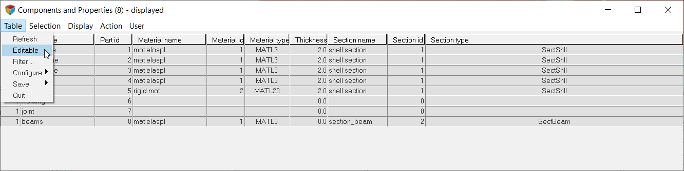
Figure 14. -
Assign the material steel to the base_frame and back_frame components.
- Select the base_frame component.
- Set Assign Values to Material name.
- Set HM-Mats to steel.
- Click Set.
- In the Confirm dialog, click Yes.
- Repeat steps 4.a through 4.e for the back_frame component.
The Material name for base_frame and back_frame is set to steel as seen in Figure 15.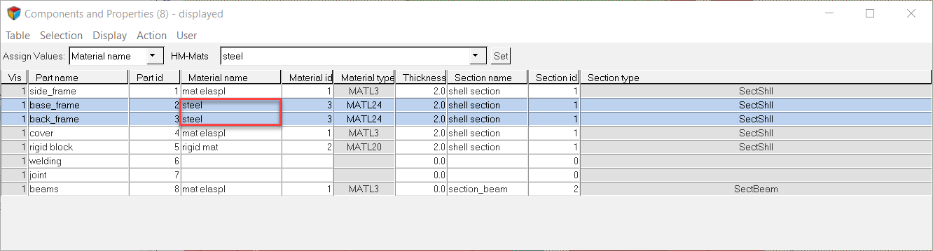
Figure 15.
Create a Beam Element
In this step, you will create a beam element, *ELEMENT_BEAM, to complete the seat's back_frame connection to the side_frame on the left side.
-
Restore a pre-defined view.
- In the Model Browser, Views folder, right-click on Beam_view and select Show from the context menu.
-
Set the current component to beams.
-
Create the beam element.
-
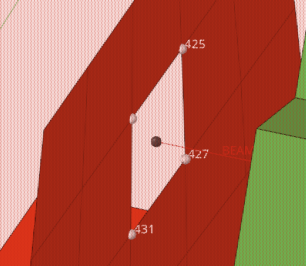
Using the node A selector, select the center node of the left nodal
rigid body as seen in Figure 16.
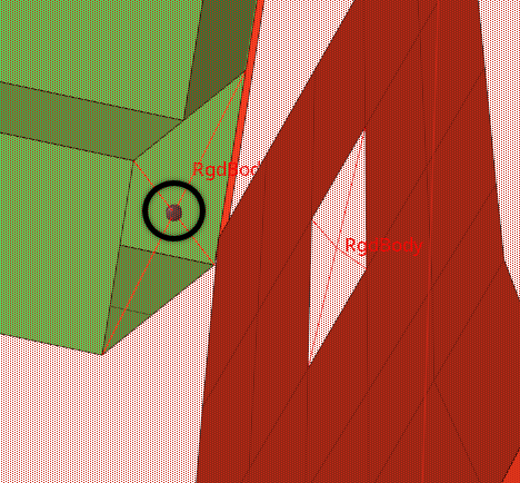
Figure 16. -
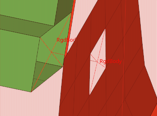
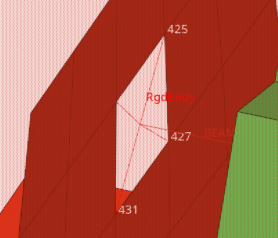
Using the node B selector, select the center node of the right nodal
rigid body as seen in Figure 17.
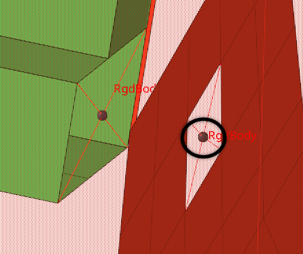
Figure 17. - Using the direction node selector, select any non-center node on one of the nodal rigid bodies.
-
Using the node A selector, select the center node of the left nodal
rigid body as seen in Figure 16.
Display Node IDs
In this step, you will display node IDs.
-
Click
 on
the Display toolbar.
The Numbers panel opens.
on
the Display toolbar.
The Numbers panel opens. - Click on.
Set the Current Component to Welding
In this step, you will set the current component to welding.
Select the RgdBody Type for the Rigid Configuration
In this step, you will select the rgdbody type for theEngineering Solutions rigid configuration.
Create the Nodal Rigid Body
Display Node IDs
In this step, you will display node IDs.
-
On the Visualization toolbar, click
 to display the model's elements as wireframe elements skin only.
- Click on.
Activate Coincident Picking
In this step, you will activate coincident picking from the graphics panel.
Set the Current Component to Joint
In this step, you will set the joint component as the current collector.
Create a Revolute Joint
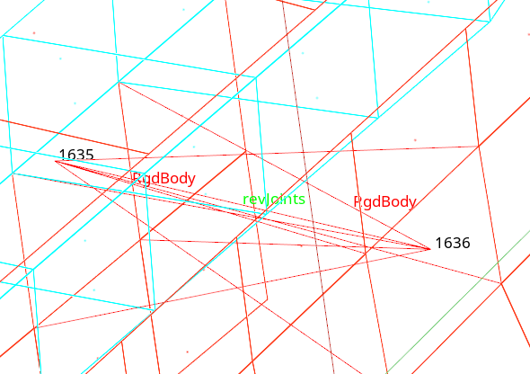
In this step, you will create a joint between two nodal rigid bodies (*CONSTRAINED_JOINT_REVOLUTE).
-
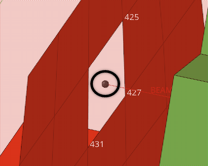
Using the node 1 selector, click node 1635.
The coincident picking mechanism displays the nodes 1635 and 1633 as seen in Figure 24.
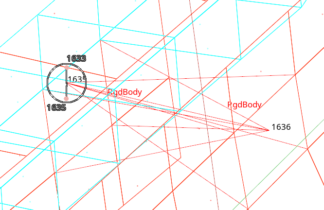
Figure 24. - Click create.
Define *DEFORMABLE_TO_RIGID
In this step, you will define *DEFORMABLE_TO_RIGID to set up the moving seat as rigid until the time of impact with the block, to reduce computation time.
-
Create an entity set that contains the base_frame, back_frame, and cover
components.
-
In the Solver Browser, right-click and select from the context menu.
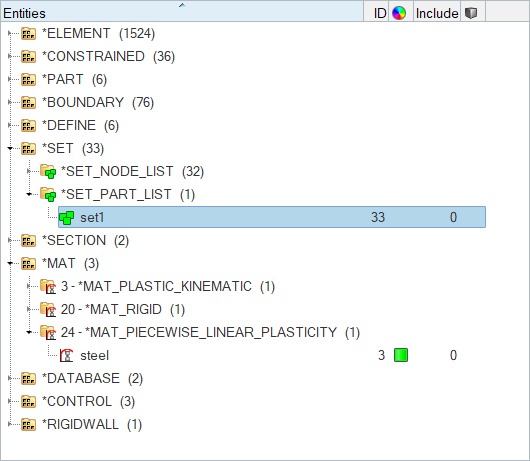
Figure 26.Engineering Solutions creates and opens a new set in the Entity Editor. -
For Entity IDs, click .
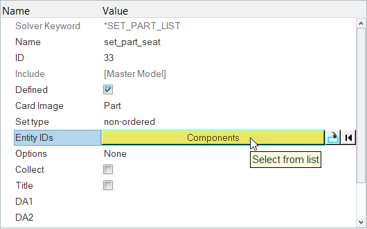
Figure 27.The Select Components dialog opens. -
In the Select Components dialog, select
base_frame,
back_frame, and cover and
then click OK.
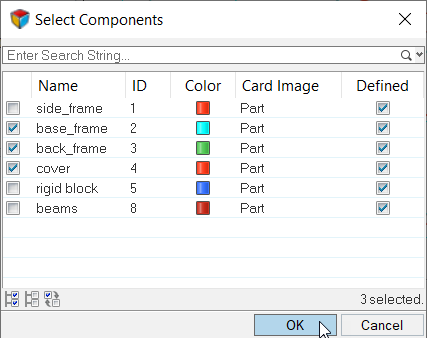
Figure 28.
-
In the Solver Browser, right-click and select from the context menu.
-
Define *DEFORMABLE_TO_RIGID to switch the deformable seat to rigid at the
beginning of the analysis.
-
In the Solver Browser, right-click and select from the context menu.
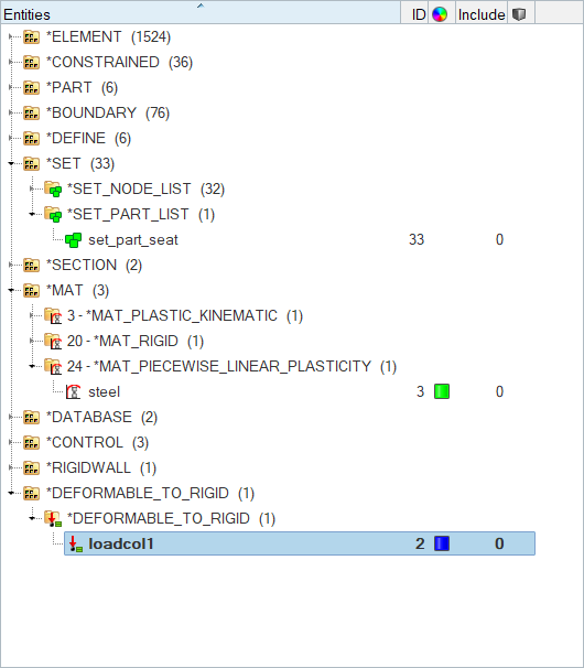
Figure 29.Engineering Solutions creates and opens a new load collector in the Entity Editor. -
For PSID, click .
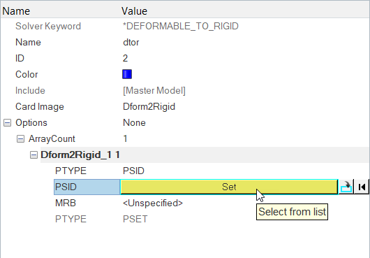
Figure 30.The Select Set dialog opens.
-
In the Solver Browser, right-click and select from the context menu.
-
Define *DEFORMABLE_TO_RIGID_AUTOMATIC to switch the rigid seat to deformable
when contact between the seat and block is detected.
-
In the Solver Browser, right-click and select from the context menu.
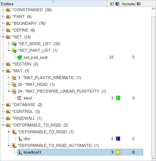
Figure 31.Engineering Solutions creates and opens a new load collector in the Entity Editor. -
Click .
Note: PSIDR2D is the part ID of the part which is switched to a rigid material.
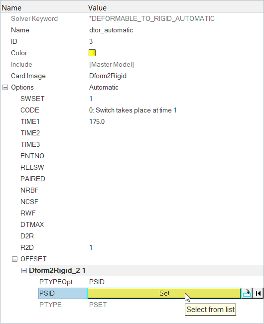
Figure 32.The Select Set dialog opens.
-
In the Solver Browser, right-click and select from the context menu.
Review Component Data
In this section, you will review the model’s component data using the Model Browser, Solver Browser, or Component Table tool.
Method 1: Use the Model Browser
In this section, you will review the model's component data using the Model Browser.
-
Display only parts of the model with a particular material and section.
-
In the Model Browser, click
 .
.
-
Right-click on steel and select
Isolate from the context menu.
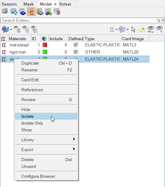
Figure 33.Engineering Solutions only displays the components that have the selected material assigned. -
Click
 ,
select a material, and scroll through the material using the up and down
arrow keys in the Model Browser to review the
materials.
The corresponding parts are automatically isolated in the view.
,
select a material, and scroll through the material using the up and down
arrow keys in the Model Browser to review the
materials.
The corresponding parts are automatically isolated in the view. -
In the Model Browser click
 .
.
-
Right-click on shell section and select
isolate from the context menu.
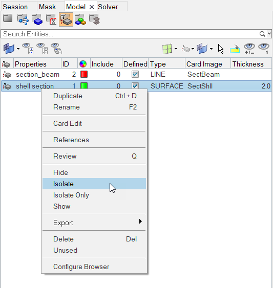
Figure 34.Engineering Solutions only displays the components that have the selected section assigned.
-
In the Model Browser, click
-
Display all components.
-
In the Model Browser, click
 .
.
-
In the Model Browser, click
-
Rename a part.
-
Renumber a part ID.
Method 2: Use the Solver Browser
In this section, you will review the model's component data using the Solver Browser.
-
Display only parts with a particular material.
- In the Model Browser, Materials folder, right-click on Steel and select Isolate from the context menu.
- In the Solver Browser, *SECTION folder, select components based on properties.
-
Display all components.
- In the Solver Browser, click the *MAT folder.
-
Rename a part.
-
Renumber a part ID.
Method 3: Use the Component Table
In this section, you will review the model's component data using the component table.
-
Display only parts with a particular material.
-
Display all components.
-
Rename a part.
-
Renumber a part ID.